MCCB vs ACB vs MCB

MCCB vs ACB vs MCB: Differences and Selection Guide

An MCCB (moulded case circuit breaker), an ACB (air circuit breaker) and an MCB (miniature circuit breaker) are three distinct classes of low-voltage protective switching devices, distinguished primarily by rated current range, interrupting (breaking) capacity, enclosure construction and the position they occupy in a distribution hierarchy — from main incomers down to final branch circuits. This guide explains, from first principles, how a specifying engineer chooses between the three using load current, prospective short-circuit current and discrimination requirements, and walks through a fully worked sizing example. The same selection logic applies whether the installation sits in a Gulf industrial park, a North African water treatment plant, a CIS power utility substation or a Sub-Saharan Africa mining facility — the physics of fault current does not change with geography, even though cable lengths, ambient temperature and grid stiffness do.

These three breaker families typically sit downstream of medium voltage switchgear and the step-down transformer, and are frequently coordinated with [protection relays](/what-is-a-medium-voltage-protection-relay-mv-protection-relay/) at the upstream MV breaker for overall system selectivity.
MCCB vs ACB vs MCB — schematic
MCCB vs ACB vs MCB — schematic.

The method: how rated current and fault current drive breaker selection

Selecting among MCB, MCCB and ACB is a two-step calculation, not a catalog guess.

Step 1 — Determine the load/rated current (In). For a three-phase load fed from a transformer or a distribution board:

I (A) = S / (√3 × V)

where S is the apparent power in VA and V is the line-to-line voltage in volts. This gives the continuous current the breaker’s frame and trip unit must carry without nuisance tripping, and is the starting point for choosing the breaker’s rated current.

Step 2 — Determine the prospective short-circuit current (Isc) at the point of installation. A simplified, transformer-limited approximation is:

Isc ≈ I_rated(transformer) / Z%

where Z% is the transformer’s per-unit short-circuit impedance expressed as a percentage. This is the fault current the breaker must be able to interrupt safely — its rated breaking capacity must be equal to or greater than this value at the point of application. Downstream of the transformer, cable and busbar impedance further reduce the prospective fault current, which is why fault levels — and therefore the required breaker class — fall as you move from the main incomer toward final branch circuits.

The breaker type is then chosen by matching: 1. Rated current range to the load/circuit current, and 2. Rated breaking capacity (and, for selectivity studies, let-through energy I²t) to the prospective fault current at that point in the network.
Selection reference
Selection reference.

Worked example: from transformer rating to breaker class at three points in the network

Transformer secondary (main LV incomer). For a 1000 kVA, 11/0.4 kV distribution transformer, the rated secondary current is:

I = S / (√3 × V) = 1,000,000 / (1.732 × 400) ≈ 1,443 A

Assuming a typical transformer short-circuit impedance of 6%, the approximate prospective fault current at the transformer terminals is:

Isc ≈ I_rated / Z% = 1,443 / 0.06 ≈ 24,050 A ≈ 24 kA

A device carrying roughly 1,443 A continuously and clearing a prospective fault near 24 kA at the main LV board sits squarely in ACB territory — air circuit breakers are built for high continuous current and high breaking capacity at main incomers and bus-tie positions, and are normally supplied in withdrawable (drawout) construction for maintenance without de-energising the busbar.

Sub-distribution board (downstream of cable/busbar impedance). Further down the network, after cable and busbar impedance has reduced the fault level, a sub-distribution panel might see a rated circuit current of around 250 A and a prospective fault current reduced to the low-to-mid tens of kA — a level still significant but below the main incomer value. This duty profile — moderate current, moulded insulating case, non-withdrawable, compact — is the classic MCCB application: feeders, motor circuits, and sub-main distribution.

Final branch circuit (lighting/socket panel). At the final distribution level, a lighting or small power circuit typically draws on the order of tens of amperes (for example, a 32 A final circuit) and the prospective fault current at that point, after further cable attenuation, is reduced to a few kA. This is the domain of the MCB — a compact, low-current, fixed (non-adjustable or minimally adjustable) device intended for simple overcurrent and short-circuit protection of final circuits, not for repeated heavy fault duty.

This progression — ACB at the top, MCCB in the middle, MCB at the final circuit — mirrors how fault current naturally decays through transformer, cable and busbar impedance as you move away from the source.

Comparison table: MCB vs MCCB vs ACB

Characteristic MCB MCCB ACB
Typical network position Final branch circuits Sub-distribution, feeders, motor circuits Main incomer, bus-tie, generator breaker
Construction Fixed, sealed miniature module Moulded insulating case Open-frame, often withdrawable (drawout)
Trip unit adjustability Fixed or minimal adjustment Thermal-magnetic or electronic, adjustable Electronic trip unit, fully adjustable (LSIG)
Continuous current role Low Low–moderate High
Breaking capacity role Low Moderate High
Maintenance under load Not applicable Limited Withdrawable design allows isolation/maintenance
Governing IEC standard IEC 60898-1 IEC 60947-2 IEC 60947-2

Note: the table expresses relative roles, not fixed numeric ratings — actual rated current and breaking capacity for a given product must always be read from its datasheet, since ranges vary by manufacturer and series.

Selection criteria and common pitfalls

  • Match frame to fault level, not just load current. A breaker sized correctly for continuous current but under-rated for prospective fault current will fail catastrophically during a short circuit. Always carry the Isc calculation through to the actual installation point, including cable and busbar impedance, not just the transformer terminal value.
  • Check discrimination (selectivity) between tiers. An ACB upstream and an MCCB downstream — or an MCCB upstream and an MCB downstream — must be coordinated so that a fault on a final circuit trips only the nearest device, not the upstream breaker. This is normally verified using manufacturer discrimination tables or time-current curve studies, and is essential wherever an upstream MV protection relay scheme also needs to remain selective with the LV side.
  • Do not use an MCB where fault levels exceed its duty. A common field error is extending MCB-protected final circuits too close to a stiff source (e.g., directly off a large transformer) without adequate cable impedance to limit the fault current — this can exceed the MCB’s short-circuit rating.
  • Withdrawable ACBs need space and maintenance planning. Drawout mechanisms require clearance for racking in/out and periodic mechanical maintenance; this should be allowed for in panel layout from the design stage.
  • Ambient temperature and altitude affect thermal trip calibration, particularly for thermal-magnetic trip units; electronic trip units in MCCBs and ACBs are generally less sensitive to ambient variation but still require correct setting verification.
  • Re-verify after any network change. Adding generation, increasing transformer size, or re-routing cables changes the prospective fault current at every downstream point — breaker selection should be revisited whenever upstream source impedance changes.

Standards

Low-voltage circuit-breaker selection in this guide is governed by two complementary IEC standards: IEC 60947-2, which covers circuit-breakers for industrial applications including both MCCBs and ACBs (rated current, breaking capacity, utilisation categories), and IEC 60898-1, which covers circuit-breakers for overcurrent protection of household and similar installations — the standard under which MCBs are rated and tested. General rules common to low-voltage switchgear and controlgear assemblies are addressed in IEC 60947-1. Where a project also involves medium voltage switchgear upstream, coordination studies typically reference the relevant IEC 62271 series for the MV side separately from the LV breaker standards above.

Related guides

See also our guides on gas-insulated switchgear, ring main units and metal-clad switchgear.

What is the main functional difference between an MCCB and an ACB?

Both are industrial circuit breakers covered by the same general standard (IEC 60947-2), but an ACB is built with an open-frame, typically withdrawable construction for high continuous current and high breaking duty at main incomers, while an MCCB uses a compact moulded insulating case and is generally applied at lower current and fault-level positions such as feeders and motor circuits.

Can an MCB be used instead of an MCCB for a feeder circuit?

Only if the feeder’s rated current and the prospective short-circuit current at that point both fall within the MCB’s rating — MCBs are designed and tested under IEC 60898-1 for lighter final-circuit duty, not for higher-current feeder or motor-circuit applications.

How do I know if I need an MCCB or an ACB at the main LV board?

Compute the transformer’s rated secondary current with I = S/(√3×V) and the approximate fault current with Isc ≈ I_rated/Z%. If the resulting continuous current and fault level are high — as at a typical main incomer — an ACB with withdrawable construction and a high breaking capacity is normally the appropriate class; lower current, lower fault-level sub-distribution points are usually served by MCCBs.

Why does fault current decrease as you move from the transformer to a final MCB circuit?

Each additional length of cable or busbar between the source and the load point adds impedance, which limits the current that can flow during a short circuit. This is why prospective fault levels — and the required breaker breaking capacity — are highest at the main incomer and progressively lower at sub-distribution and final-circuit levels.

What does “discrimination” or “selectivity” mean between MCB, MCCB and ACB tiers?

It means that when a fault occurs, only the breaker closest to the fault should open, while upstream breakers (MCCB, then ACB) remain closed to keep the rest of the installation energised. Achieving this requires coordinating trip settings and time-current characteristics across all three tiers, verified against manufacturer discrimination data.

Is a withdrawable (drawout) design unique to ACBs?

Withdrawable construction is most commonly associated with ACBs because of their role at main incomers where maintenance without full shutdown is valuable; some MCCB ranges also offer withdrawable or plug-in options, but it is not a standard feature for MCBs, which are fixed devices.

Which IEC standard applies to each breaker type?

MCCBs and ACBs are both tested and rated under IEC 60947-2 (circuit-breakers for industrial applications), while MCBs follow IEC 60898-1 (circuit-breakers for overcurrent protection of household and similar installations). General assembly rules are covered separately in IEC 60947-1.

Looking for low voltage switchgear?

Looking for high-quality low voltage switchgear? We provide expert engineering support and reliable products for all your medium voltage needs.

For quotations and requests: info@electricistanbul.com

WhatsApp: +90 501 076 69 91
Detuned Reactor Power Factor Correction

Detuned Reactor Power Factor Correction: Harmonics, Sizing & Tuning Guide

A detuned reactor is a series-connected inductor placed between a power factor correction (PFC) capacitor and the busbar to shift the capacitor-reactor branch’s resonant frequency below the lowest significant harmonic present on the network, preventing harmonic amplification while still supplying reactive power at fundamental frequency. This guide walks through why plain (undetuned) capacitor banks fail in harmonic-rich installations, the tuning-factor formula used to size a detuned reactor, a fully worked numerical example, a comparison table of common tuning classes, selection pitfalls, and the governing standards. It is written for engineers specifying power factor correction and capacitor bank systems across the Middle East and Gulf (including Egypt and Saudi Arabia), North Africa, CIS, and Sub-Saharan Africa, where variable frequency drives, rectifiers, and UPS loads are increasingly common on medium-voltage and low-voltage industrial feeders.

Detuned Reactor Power Factor Correction — schematic
Detuned Reactor Power Factor Correction — schematic.

Why Plain Capacitor Banks Fail in Harmonic Environments

A capacitor bank connected directly across a busbar — with no series reactor — forms a parallel LC resonant circuit with the upstream source/transformer inductance. If a harmonic current source (a variable frequency drive, DC rectifier, arc furnace, or UPS front end) injects current at a frequency close to this parallel resonance point, the resonant circuit amplifies that harmonic voltage and current, sometimes by a large multiple of the injected value. The results are well known to maintenance engineers: capacitor fuse blowing, dielectric overheating, nuisance tripping of protection relays, and in severe cases capacitor can rupture. The fifth harmonic (250 Hz on a 50 Hz system) generated by six-pulse rectifiers and drives is the most common culprit because plain PFC banks on transformer-fed LV/MV busbars frequently resonate close to this order.

A detuned reactor solves this by deliberately detuning the capacitor-reactor branch so its own series resonance sits below the lowest harmonic of concern. Below that point the branch is inductive, not capacitive, for all relevant harmonic frequencies, so it cannot form a parallel resonance with the upstream network impedance at those harmonics — it instead acts as a harmonic sink, attenuating rather than amplifying.

Selection reference
Selection reference.

The Tuning Formula

The design variable is the tuning factor p, expressed as a percentage, which relates the reactor’s reactance to the capacitor’s reactance at fundamental frequency:

p (%) = (X_L / X_C) × 100

where X_L is the reactor reactance and X_C is the capacitor reactance at the fundamental (50 Hz or 60 Hz).

The resulting resonant frequency of the detuned branch is:

f_r = f_n / √p (with p expressed as a fraction, e.g. 0.07 for 7%)

or equivalently, expressed as a tuning order n_r (the harmonic order at which the branch resonates):

n_r = 1 / √p

Design practice is to choose p so that n_r falls below the lowest harmonic order actually present on the system — commonly below the 5th harmonic, which corresponds to tuning factors in roughly the 5.7%–7% range, or below the 3rd harmonic for installations with significant triplen harmonic content, which requires a higher tuning factor (around 13%–14%).

Because the series reactor adds inductive reactance, it also raises the operating voltage across the capacitor above the pure bus voltage, and it reduces the effective reactive power delivered at fundamental frequency compared with the reactor’s nameplate kvar rating. Both effects must be accounted for when selecting capacitor voltage rating and bank kvar, which is why detuned-reactor-capacitor assemblies are supplied and rated as matched sets rather than reactors and capacitors chosen independently.

Worked Example: Sizing a Detuned Reactor for a 5th-Harmonic Environment

Consider a 400 V, 50 Hz industrial busbar supplying a mix of linear loads and variable frequency drives, where the dominant harmonic is the 5th (250 Hz). The plant requires a capacitor bank rated at 300 kvar at 400 V.

Step 1 — Select the tuning factor. To ensure the branch resonates below the 5th harmonic, choose p = 7% (0.07), a common choice for 5th-harmonic-dominant networks.

Step 2 — Check the resulting tuning order. n_r = 1/√p = 1/√0.07 ≈ 1/0.2646 ≈ 3.78

For example, a tuning order of about 3.78 sits safely below the 5th harmonic order of 5, confirming the branch will present inductive (non-resonant) behaviour at the 5th harmonic and above.

Step 3 — Find the resonant frequency. f_r = f_n × n_r = 50 Hz × 3.78 ≈ 189 Hz

For example, this 189 Hz resonance point is well clear of the 250 Hz fifth-harmonic current injected by the drives, and also clear of the fundamental 50 Hz, so the branch neither resonates with the harmonic source nor interacts adversely with the fundamental.

Step 4 — Determine the capacitor reactance at 50 Hz. For a 300 kvar, 400 V capacitor bank: X_C = V² / Q = (400)² / 300,000 = 160,000 / 300,000 ≈ 0.533 Ω

Step 5 — Determine the required reactor reactance. X_L = p × X_C = 0.07 × 0.533 ≈ 0.0373 Ω

Step 6 — Convert to inductance. L = X_L / (2π × f_n) = 0.0373 / (2π × 50) ≈ 0.0373 / 314.16 ≈ 118.8 µH

This worked calculation illustrates the sizing logic; in practice the reactor and capacitor are purchased as a matched, factory-tuned assembly rated for the specific p value, busbar voltage, and kvar step, with the capacitor’s nominal voltage rating increased to compensate for the voltage rise across the series reactor at fundamental frequency.

For reference, the rated full-load current draw of the capacitor step itself follows the standard three-phase formula I = Q / (√3 × V). For example, for the 300 kvar / 400 V bank above: I = 300,000 / (1.732 × 400) ≈ 300,000 / 692.8 ≈ 433 A, a useful cross-check figure when selecting protection relay settings, cabling, and contactors for the capacitor step — see our protection relay selection guidance for related overcurrent and capacitor-protection settings.

Comparison Table: Common Detuned Reactor Tuning Classes

Tuning factor p Approx. tuning order n_r Approx. resonant frequency (50 Hz system) Typical application driver
5.67% ≈ 4.2 ≈ 210 Hz Light 5th-harmonic content, conservative margin below 250 Hz
7% ≈ 3.78 ≈ 189 Hz Standard choice for installations dominated by 6-pulse VFDs/rectifiers (5th harmonic)
14% ≈ 2.67 ≈ 134 Hz Networks with significant 3rd-harmonic (triplen) content, e.g. heavy single-phase non-linear loads

All values above are derived from the tuning formula n_r = 1/√p and f_r = f_n × n_r, shown as worked illustrative calculations, not fixed product specifications.

Selection Criteria and Common Pitfalls

Match the tuning factor to the dominant harmonic order, not just the “standard” value. A network with strong 3rd-harmonic content (common where large single-phase non-linear loads unbalance the system) needs a higher p (around 13–14%) than a network dominated purely by 6-pulse drive 5th-harmonic injection (around 7%). Installing a 7%-tuned bank on a 3rd-harmonic-rich network leaves the branch resonant close to the 3rd harmonic, defeating the purpose.

Uprate the capacitor’s voltage rating, not just the reactor. Because the series reactor causes a voltage rise across the capacitor terminals relative to busbar voltage, capacitors used in detuned assemblies must carry a higher voltage rating than the bus voltage; using a plain capacitor rated only for bus voltage in a detuned assembly will lead to premature dielectric ageing or failure.

Do not retrofit a detuned reactor onto an existing plain capacitor bank without re-engineering. The reactor changes the effective kvar delivered, the inrush and energisation behaviour, the required capacitor voltage class, and the thermal design of the enclosure. Reactor and capacitor should be specified, and ideally supplied, as a matched set.

Check reactor thermal withstand and cooling. Detuned reactors carry continuous harmonic current superimposed on the fundamental reactive current and dissipate real power as heat; ventilation and ambient temperature derating must be part of the enclosure design, particularly in high-ambient GEO regions such as the Gulf and Sub-Saharan Africa.

Coordinate with transformer impedance. The upstream transformer’s source impedance interacts with the detuned branch and with other harmonic sources on the same busbar; for installations with heavy harmonic loads, a harmonic/power-quality study referencing the plant’s transformer rating is advisable — see our transformer hub page for related sizing background.

Verify with protection and monitoring. Capacitor step protection relays should be set to account for the additional harmonic current the reactor is designed to carry, not just fundamental-frequency current, and should include voltage and current THD monitoring where available.

Consider switchgear interaction. Capacitor banks are typically switched via dedicated contactors or circuit-breakers within MV or LV switchgear; switching transients (inrush, restrike) must be evaluated alongside harmonic tuning when the bank is part of an automatic power factor correction panel.

Standards and Compliance

Design and testing of shunt power capacitors used in power factor correction, including considerations for harmonic duty, are governed by the IEC 60871 series for medium-voltage shunt power capacitors, while series reactors used for detuning are generally assessed under the general reactor standard IEC 60076-6 (power transformers — reactors) framework and relevant national/plant harmonic limit guidance such as IEEE 519 for harmonic current and voltage distortion limits at the point of common coupling. Where a formal standard reference for a specific component is not available, qualitative engineering judgement based on the tuning-factor method above should guide the design, supported by a site harmonic measurement or study.

Related guides

See also our guides on medium voltage switchgear, gas-insulated switchgear and ring main units.

What is a detuned reactor in power factor correction?

A detuned reactor is a series inductor connected with a PFC capacitor so that the combined branch’s resonant frequency sits below the lowest significant harmonic on the network, preventing harmonic resonance amplification while the capacitor still supplies reactive power at fundamental frequency.

Why does a plain capacitor bank need protection from harmonics?

A plain capacitor bank connected directly to a busbar can form a parallel resonant circuit with the source impedance; if a harmonic current source injects current near that resonant frequency, voltage and current at that harmonic can be amplified, stressing capacitors, fuses, and nearby equipment.

What tuning factor should I use for a 5th-harmonic dominant load?

A tuning factor around 7% is a common choice for networks dominated by 6-pulse variable frequency drives or rectifiers, giving a tuning order below the 5th harmonic as shown in the worked example above.

Why is a higher tuning factor needed for 3rd-harmonic content?

Third-harmonic currents are lower in frequency than the 5th, so the detuned branch must resonate at an even lower frequency to stay clear of them, which requires a larger series reactance and therefore a higher tuning factor, typically in the 13–14% range.

Can I add a detuned reactor to an existing capacitor bank?

Not as a simple retrofit — the reactor changes the voltage seen by the capacitor, the effective delivered kvar, and the thermal and protection requirements, so the reactor and capacitor should be re-engineered and ideally supplied as a matched assembly.

Does a detuned reactor reduce the reactive power delivered by the capacitor bank?

Yes — because the reactor’s inductive reactance opposes part of the capacitor’s reactance at fundamental frequency, the net kvar delivered to the bus is lower than the capacitor’s own nameplate rating, which must be accounted for during bank sizing.

What standards apply to detuned reactor and capacitor bank design?

Shunt power capacitors are generally assessed against the IEC 60871 series, series reactors against the IEC 60076-6 reactor framework, and overall harmonic distortion limits against guidance such as IEEE 519, alongside any applicable plant-specific or utility harmonic limits.

Looking for power factor correction and capacitor banks?

Looking for high-quality power factor correction and capacitor banks? We provide expert engineering support and reliable products for all your medium voltage needs.

For quotations and requests: info@electricistanbul.com

WhatsApp: +90 501 076 69 91
Automatic vs Fixed Power Factor Correction

Automatic vs Fixed Power Factor Correction: Sizing, Calculation and Selection Guide

“`

Automatic power factor correction (APFC) is an engineering method that uses a controller to switch capacitor steps in and out of an electrical network in real time, keeping the power factor close to a target value as the load varies, whereas fixed power factor correction applies a constant, non-switched capacitor bank sized for one assumed operating condition. This guide explains the underlying reactive-power math, walks through a fully worked sizing example, compares fixed and automatic approaches in a decision table, and outlines the selection criteria, standards references, and common pitfalls that medium-voltage engineers face when specifying correction equipment. It is written for engineers, procurement teams and EPC contractors working across the Middle East and Gulf region including Egypt and Saudi Arabia, North Africa, CIS countries, and Sub-Saharan Africa, where industrial and utility loads frequently carry poor power factor due to motor-heavy, transformer-heavy or variable-frequency-drive-rich installations.

Automatic vs Fixed Power Factor Correction — schematic
Automatic vs Fixed Power Factor Correction — schematic.

Why power factor correction matters

Most industrial and commercial electrical loads — induction motors, transformers, arc furnaces, welding sets, and variable-frequency drives — are inductive. An inductive load draws not only active power (kW), which does real work, but also reactive power (kVAr), which is needed to sustain magnetic fields in motors and transformers but performs no useful work at the load. The vector sum of active and reactive power is apparent power (kVA), and the ratio of active power to apparent power is the power factor:

PF = kW / kVA = cos(φ)

A low power factor means the network, transformers, cables and switchgear must carry more current than strictly necessary to deliver the same amount of useful work, which increases I²R losses, reduces available transformer and cable capacity, and in many jurisdictions triggers a reactive-energy penalty on the utility bill. Correcting the power factor by installing capacitor banks that supply leading reactive power locally — close to the load — cancels out part of the inductive reactive demand drawn from the grid, reduces the total current, frees up capacity, and removes or reduces the penalty.

The central engineering question is not whether to correct power factor, but how: with a fixed bank sized for an average or worst-case condition, or with an automatic bank that tracks the load continuously.

Selection reference
Selection reference.

The method / formula

The reactive power required to raise the power factor from an existing value to a target value is derived from the active power and the tangent of the phase angle at each condition:

Q(required) = P × (tan φ₁ − tan φ₂)

Where: – P = active power of the load, in kW – φ₁ = phase angle corresponding to the existing (uncorrected) power factor, where cos φ₁ = PF₁ – φ₂ = phase angle corresponding to the target (corrected) power factor, where cos φ₂ = PF₂ – Q(required) = capacitive reactive power to be installed, in kVAr

This formula is the standard first-principles tool used for both fixed-bank sizing (one calculation, one fixed PF₁) and automatic-bank sizing (a range of PF₁ values across the load profile, corrected by a multi-step bank under controller supervision).

The related current and apparent-power relationships for a three-phase system are:

  • S (kVA) = √3 × V(line, kV) × I(A)
  • I (A) = S / (√3 × V)
  • Q (kVAr) generated by a capacitor bank reduces S proportionally as PF improves at constant P.

Worked example with computed numbers

Consider an industrial facility with an active load of 500 kW operating at an existing (uncorrected) power factor of 0.75 lagging. The target is to raise the power factor to 0.95 lagging to avoid a utility reactive-energy penalty and recover transformer capacity.

Step 1 — Find the phase angles. For PF₁ = 0.75, φ₁ = cos⁻¹(0.75) ≈ 41.4°, so tan φ₁ ≈ 0.882. For PF₂ = 0.95, φ₂ = cos⁻¹(0.95) ≈ 18.2°, so tan φ₂ ≈ 0.329.

Step 2 — Apply the formula. Q(required) = P × (tan φ₁ − tan φ₂) = 500 × (0.882 − 0.329) = 500 × 0.553 ≈ 276.5 kVAr

So a capacitor bank rated at approximately 275–280 kVAr (in practice rounded to a standard step combination, e.g. 5 × 56 kVAr or similar) would raise the power factor from 0.75 to 0.95 at this single operating point.

Step 3 — Check the current reduction. At PF₁ = 0.75: S₁ = P / PF₁ = 500 / 0.75 ≈ 666.7 kVA At PF₂ = 0.95: S₂ = P / PF₂ = 500 / 0.95 ≈ 526.3 kVA

For a 415 V three-phase low-voltage feeder: I₁ = S₁ / (√3 × V) = 666.7 / (1.732 × 0.415) ≈ 927 A I₂ = S₂ / (√3 × V) = 526.3 / (1.732 × 0.415) ≈ 732 A

This represents a current reduction of roughly 21% for the same real power delivered, directly translating into lower cable and transformer loading.

Step 4 — Why “automatic” matters here. The 276.5 kVAr figure above is correct only at the instant the load is exactly 500 kW at PF 0.75. If the plant load varies — for example dropping to 200 kW overnight with lightly loaded motors — the same fixed 276.5 kVAr bank would now over-correct the circuit into a leading power factor, which can cause overvoltage, increased losses, and even resonance risk with background harmonics. An automatic controller, sensing the instantaneous PF and load, would switch out several steps of the bank, leaving only the kVAr needed for the night-time load. This is the fundamental engineering reason automatic correction exists: the formula above is a snapshot calculation, but real loads are a time series.

Fixed vs automatic correction — comparison table

Criterion Fixed power factor correction Automatic power factor correction
Control method Permanently connected capacitor bank, no switching Controller (relay) measures PF/kVAr continuously and switches capacitor steps via contactors or thyristor switches
Best suited for Constant loads (e.g. a single large motor, a continuously loaded transformer) Variable loads (e.g. multi-motor plants, workshops, commercial buildings with load cycles)
Over-correction risk High, if load drops below the design point Low — controller de-steps capacitors as load falls
Under-correction risk High, if load rises above the design point Low — controller adds steps as load rises
Harmonic/resonance sensitivity Fixed exposure at all load levels Exposure limited to the time steps are connected; still requires detuning reactors if harmonics present
Capital cost Lower (no controller, fewer switching devices) Higher (controller, contactors/thyristor modules, enclosure)
Maintenance complexity Simple Moderate — controller, switching devices require periodic checks
Typical connection point Directly at a constant load (motor terminals, transformer secondary) Main LV/MV switchboard, bus-connected, serving multiple variable loads

Selection criteria and sizing pitfalls

1. Characterise the load profile before choosing. A fixed bank is only appropriate when the reactive demand is genuinely stable — for instance, a dedicated capacitor directly across a constantly running motor, sized using the same Q = P × (tan φ₁ − tan φ�2) formula but at the motor’s own nameplate operating point. Any facility with cyclical, shift-based, or seasonal load variation should default to automatic correction.

2. Size in realistic steps, not one big block. Automatic banks are built from multiple capacitor steps (commonly arranged in unequal or equal ratios) so the controller can approach the target PF closely without large single-step jumps that cause voltage transients. Step switching should respect minimum switching intervals to protect capacitor and contactor life and avoid repeated inrush.

3. Never ignore harmonics. Both fixed and automatic banks that are solidly connected (undetuned) can resonate with background harmonic currents from VFDs, UPS systems, or rectifiers, amplifying rather than reducing distortion. Where significant harmonic sources are present, detuned (reactor-protected) banks or active filtering should be evaluated alongside the PF correction design — this assessment belongs in the broader protection and power-quality study for the installation. See our medium-voltage switchgear hub for how correction equipment interfaces with incoming breakers and busbars.

4. Coordinate with protection and switching devices. Capacitor banks draw inrush current on switching and must be protected and interlocked correctly; this coordination is normally handled through a dedicated protection relay function and appropriately rated switching devices, not through the capacitor controller alone.

5. Re-check transformer loading after correction. Reduced apparent power (kVA) after correction effectively frees up transformer headroom; this is a legitimate design input when reviewing transformer capacity for future load growth, but the transformer’s own rating and impedance should still be verified independently.

6. Verify target PF against the actual tariff/penalty structure. Some utilities penalise PF below a threshold, others reward PF above a target; the design target (0.90, 0.95, unity, etc.) should be an input from the tariff review, not an arbitrary engineering default.

Standards and compliance framework

Shunt power capacitors for power factor correction are generally specified and tested against IEC 60871 (shunt capacitors for a.c. power systems above 1 kV) for medium-voltage applications, while automatic power factor correction equipment incorporating controllers, switching contactors, and low-voltage capacitor banks is commonly built to IEC 61921 (low-voltage power factor correction banks) and related low-voltage switchgear assembly standards for the enclosure and switching components. Capacitor-switching contactors and controllers should be selected according to their rated duty for frequent capacitive switching, as recommended in the governing capacitor and switchgear standards, rather than by generic contactor ratings. Engineers should also account for applicable national grid codes or utility technical connection requirements, which often define the minimum power factor to be maintained at the point of common coupling.

Related guides

See also our guides on gas-insulated switchgear, ring main units and metal-clad switchgear.

What is the difference between fixed and automatic power factor correction?

Fixed correction connects a constant capacitor bank sized for one assumed load condition, while automatic correction uses a controller to switch capacitor steps on and off in response to the real-time load, keeping the power factor close to a target across varying operating conditions.

How do I calculate the kVAr needed for power factor correction?

Use Q = P × (tan φ₁ − tan φ₂), where P is the active load in kW, φ₁ is the angle for the existing power factor, and φ₂ is the angle for the target power factor. The worked example above shows this calculation step by step for a 500 kW load moving from PF 0.75 to PF 0.95.

When is a fixed capacitor bank still the right choice?

When reactive demand is genuinely constant, such as a capacitor dedicated to a single continuously running motor or a steadily loaded transformer, a fixed bank sized at that one operating point can be simpler and more economical than automatic correction.

Can over-correction with a fixed bank cause problems?

Yes — if the load drops below the design point, a fixed bank can push the power factor leading, which may cause overvoltage at light load, increased system losses, and higher sensitivity to harmonic resonance; automatic correction avoids this by de-stepping capacitors as load falls.

Does power factor correction affect transformer and cable sizing?

Yes — reducing reactive current for the same active power lowers the total current (as shown in the worked example’s roughly 21% current reduction), which reduces I²R losses and can free up transformer and cable capacity for additional load.

Do I need detuning reactors with an automatic capacitor bank?

If the installation has significant harmonic-producing loads such as VFDs or rectifiers, detuned or filtered capacitor banks should be evaluated to avoid resonance; a plain automatic bank without reactors is suitable mainly where harmonic content is low.

What standards govern power factor correction equipment?

Medium-voltage shunt capacitors are typically referenced against IEC 60871, and low-voltage automatic power factor correction banks against IEC 61921, alongside applicable utility grid-code requirements for minimum power factor at the connection point. “`

Looking for power factor correction and capacitor banks?

Looking for high-quality power factor correction and capacitor banks? We provide expert engineering support and reliable products for all your medium voltage needs.

For quotations and requests: info@electricistanbul.com

WhatsApp: +90 501 076 69 91
Power Factor Correction Panel Troubleshooting

Power Factor Correction Panel Troubleshooting: A Fault-Finding and Calculation Guide

A power factor correction (PFC) panel is an assembly of capacitor steps, contactors or thyristor switches, detuning reactors, and a controller that automatically injects reactive power (kVAr) to bring a facility’s power factor close to unity, and troubleshooting it means systematically isolating whether a fault lies in the capacitors, the switching devices, the controller logic, or the supply network itself. This guide walks through the governing formulas, a fully worked kVAr sizing and fault-current example, a structured fault-diagnosis table, and the IEC references that apply to capacitor banks and their protection — content that is directly relevant for utilities and industrial plants across the Middle East and Gulf region including Egypt and Saudi Arabia, North Africa, CIS countries, and Sub-Saharan Africa, where voltage fluctuations and harmonic-rich loads make PFC panels particularly fault-prone.

Power Factor Correction Panel Troubleshooting — schematic
Power Factor Correction Panel Troubleshooting — schematic.

Why Power Factor Correction Faults Matter

A poorly functioning PFC panel does more than fail to correct power factor — it can actively damage the installation. Common consequences of undetected faults include:

  • Reactive power billing penalties when the panel under-compensates.
  • Leading power factor and overvoltage when the panel over-compensates during light load.
  • Capacitor case rupture or fuse operation from sustained overcurrent or harmonic resonance.
  • Nuisance tripping of upstream breakers due to inrush current on contactor switching.
  • Thermal stress on detuning reactors leading to insulation failure.

Because the panel sits electrically close to switchgear, protection relays, and sometimes directly on transformer secondaries, a capacitor fault can also distort measurements used by protection relays, so troubleshooting should always consider the panel’s interaction with the wider MV/LV protection scheme — see our switchgear and protection relay hub pages for related fault-clearing concepts.

Selection reference
Selection reference.

The Core Method: Reactive Power Balance and Reconstructing the Fault

The starting point for both sizing and diagnosis is the reactive power triangle:

Q (kVAr) = P × (tanφ₁ − tanφ₂)

where P is active power (kW), φ₁ is the existing phase angle (from the measured power factor), and φ₂ is the target phase angle (from the desired power factor).

For diagnosing an in-service panel, the key relationships an engineer checks step by step are:

  1. Rated capacitor current: I_c = Q / (√3 × V), used to confirm whether a step is actually drawing its expected current.
  2. Capacitance from nameplate kVAr: C = Q / (2π × f × V²), used to verify whether a capacitor has degraded (capacitance loss shows up as reduced current draw for the same voltage).
  3. Resonance frequency check against detuning reactors: f_r = f × √(Q_sc / Q_c), comparing network short-circuit power to the capacitor bank’s reactive power, to confirm the installation isn’t exposed to harmonic resonance.
  4. Step switching inrush estimate, relevant for selecting contactors and explaining nuisance trips on energization.

These four checks, applied in sequence, cover the overwhelming majority of real PFC panel complaints: under/over-compensation, capacitor degradation, harmonic-driven failures, and switching-related trips.

Worked Example: Sizing and Verifying a PFC Step

Consider a plant load of 500 kW operating at an existing power factor of 0.75 lagging, and the target is to raise it to 0.95 lagging.

Step 1 — Find the phase angles. φ₁ = arccos(0.75) ≈ 41.4°, so tanφ₁ ≈ 0.882. φ₂ = arccos(0.95) ≈ 18.2°, so tanφ₂ ≈ 0.329.

Step 2 — Apply the reactive power balance formula. Q = P × (tanφ₁ − tanφ₂) = 500 × (0.882 − 0.329) ≈ 500 × 0.553 ≈ 276.5 kVAr.

So the panel needs roughly 277 kVAr of correction, which in a typical step configuration might be realized as, for example, 4 steps of about 70 kVAr each (an illustrative split, not a fixed rule — actual step sizing also depends on load variability).

Step 3 — Check the rated current of one 70 kVAr step on a 400 V LV bus. I_c = Q / (√3 × V) = 70,000 / (1.732 × 400) ≈ 70,000 / 692.8 ≈ 101 A.

If, during troubleshooting, a clamp-meter reading on that step shows only around 70–80 A instead of the expected ≈101 A, this is a strong indicator of partial capacitor degradation (dielectric aging or a blown internal fuse element reducing effective capacitance), not a supply-voltage issue — because a simple undervoltage would move current only modestly, whereas noticeably below the calculated value more consistently points to lost capacitance.

Step 4 — Resonance sanity check. If the upstream transformer has a short-circuit power Q_sc much larger than the capacitor bank’s Q_c, the natural resonance order stays high and away from common harmonic orders (5th, 7th). If Q_sc and Q_c are close in magnitude, f_r = f × √(Q_sc/Q_c) can land near a dominant harmonic produced by variable-speed drives or rectifier loads, which is why detuned reactors (tuned below the 5th harmonic, commonly described qualitatively rather than by a fixed universal figure since it depends on site harmonic content) are specified for installations with significant nonlinear loads.

This four-step method — compute expected Q, compute expected current, compare measured to expected, then check resonance exposure — is the backbone of almost every PFC troubleshooting visit.

Fault Diagnosis Table

Symptom observed Likely root cause Diagnostic check Typical corrective action
Power factor stays lagging below target Steps not switching in / controller setpoint wrong Verify controller target cosφ and step enable status Reconfigure controller, check contactor coil circuit
Power factor swings to leading at light load Over-compensation, steps not de-switching fast enough Compare switched kVAr to actual load reactive demand over time Reduce step size granularity, adjust controller time delay
Capacitor fuse operates repeatedly Harmonic overcurrent or resonance Measure harmonic spectrum, compute f_r vs Q_sc/Q_c ratio Install or retune detuning reactors
Capacitor case bulging / leaking Sustained overvoltage or internal dielectric failure Check supply voltage profile and capacitor can temperature Replace capacitor unit, verify ventilation
Step current reads below calculated I_c Partial internal capacitor failure (lost capacitance) Recalculate I_c = Q/(√3·V) and compare to clamp-meter reading Replace degraded capacitor unit
Contactor chatter or nuisance trip on switching Inrush current exceeding contactor rating Review inrush estimate vs contactor make/break capability Use inrush-limiting contactors or sequential switching
Controller shows wrong power factor reading CT polarity or wiring error on measurement input Verify CT ratio, phase orientation, and burden Correct CT wiring, re-commission controller

Selection Criteria and Common Pitfalls

When specifying or troubleshooting a PFC panel, engineers should keep the following in mind:

  • Step resolution vs load variability. Fine step resolution reduces over/under-compensation swings but adds switching device count and cost.
  • Detuned vs undetuned banks. Any site with variable-frequency drives, UPS systems, or rectifier loads should default to detuned (reactor-equipped) banks to avoid harmonic resonance, described qualitatively here since the exact tuning order is site-specific.
  • Switching technology. Contactor-based switching is economical for slower-varying loads; thyristor (static) switching is preferred where load reactive demand changes rapidly, to avoid transient overvoltage and mechanical wear.
  • Temperature and ventilation. Capacitor lifespan is strongly temperature-dependent; panels installed in poorly ventilated rooms in hot climates are a recurring failure mode in the GEO region described above.
  • Protection coordination. Capacitor fuses and any upstream breaker or relay must be coordinated so that a single degraded capacitor can be isolated without de-energizing the whole bank — a concept shared with broader MV protection relay coordination practice.
  • Common pitfall: assuming a tripped fuse is a nuisance and simply replacing it without checking harmonic content or resonance — repeated fuse operation almost always signals an underlying resonance or overvoltage condition that will recur.
  • Common pitfall: sizing kVAr purely from nameplate transformer rating instead of actual measured reactive demand, which routinely leads to over-compensation at partial load.

Standards and Compliance Notes

Capacitor units, banks, and their series reactors used in power factor correction applications are generally addressed by the IEC 60871 series for shunt power capacitors, while IEC 61921 addresses low-voltage power factor correction banks specifically. Where PFC equipment is integrated with MV switchgear, the switchgear enclosure and switching device design should still comply with the relevant MV switchgear standards referenced on our switchgear pages, while protection relays coordinating with capacitor banks follow general protection relay application practice rather than capacitor-specific standards. Where a national grid code imposes power-factor penalty thresholds, the controller setpoint (target cosφ) should be selected to satisfy that code with margin.

Related guides

See also our guides on medium voltage switchgear, gas-insulated switchgear and ring main units.

What is the first check to make when a PFC panel shows the wrong power factor on its controller?

Verify the current transformer (CT) wiring and ratio feeding the controller before suspecting the capacitors themselves, since a reversed or mis-rated CT is a very common cause of an apparently “faulty” power factor reading.

How do I know if a capacitor step has actually failed versus just a supply voltage sag?

Recalculate the expected step current using I_c = Q/(√3×V) with the actual measured supply voltage, then compare to the clamp-meter reading; a deviation far beyond what the voltage sag alone would explain points to lost capacitance inside the unit.

Why does my capacitor bank keep blowing fuses even though the load hasn’t changed?

Repeated fuse operation without a load change is a classic sign of harmonic resonance between the capacitor bank and the supply network; check whether the bank is detuned and whether nonlinear loads (drives, rectifiers) have been added nearby.

Should I always use detuned reactors with power factor correction capacitors?

Not always — if the facility’s load is purely linear with negligible harmonic content, an undetuned bank can be adequate, but any site with variable-frequency drives or significant electronic loads should use detuned (reactor-equipped) banks as a precaution.

What causes a leading power factor after correction?

Leading power factor typically results from over-compensation, where too many capacitor steps remain switched in during light-load periods; reviewing the controller’s switching delay and step granularity usually resolves it.

Can a PFC panel fault affect upstream protection relays?

Yes — capacitor switching transients and harmonic distortion can influence current and voltage measurements used by protection relays, so panel faults should be evaluated alongside the overall protection coordination scheme, not in isolation.

How often should a PFC panel be inspected to prevent faults?

While inspection intervals depend on site conditions and load duty, routine checks of capacitance (via current measurement), fuse condition, and contactor operation are standard preventive maintenance practice for these panels.

Looking for power factor correction and capacitor banks?

Looking for high-quality power factor correction and capacitor banks? We provide expert engineering support and reliable products for all your medium voltage needs.

For quotations and requests: info@electricistanbul.com

WhatsApp: +90 501 076 69 91
Capacitor Bank kVAr Sizing

Capacitor Bank kVAr Sizing — Worked Example

“`

Capacitor bank kVAr sizing is the engineering calculation that determines the reactive power compensation (in kVAr) required to raise a facility’s power factor from an existing lagging value to a target value, based on the active power load and the two corresponding power factor angles. This guide walks through the governing formula, a complete worked example for a medium-voltage industrial load, a comparison table of sizing steps, and the selection pitfalls engineers should watch for. It is written for plant electrical engineers, EPC contractors, and procurement teams across the Middle East and Gulf region (including Egypt and Saudi Arabia), North Africa, CIS, and Sub-Saharan Africa who need to specify power factor correction equipment correctly the first time.

Capacitor banks are frequently paired with medium-voltage switchgear for protection and switching, coordinated with [protection relays](/what-is-a-medium-voltage-protection-relay-mv-protection-relay/) for overcurrent and capacitor-specific protection, and installed downstream of distribution transformers where the reactive demand originates.

Capacitor Bank kVAr Sizing — schematic
Capacitor Bank kVAr Sizing — schematic.

Why kVAr sizing matters

A plant operating at a low (poor) power factor draws more apparent current from the utility than the active power it actually consumes. This excess current increases I²R losses in cables and transformers, causes avoidable voltage drop, and in most tariff structures triggers a reactive-energy penalty on the utility bill. Correct capacitor bank sizing solves this by injecting leading reactive power (kVAr) that cancels part of the lagging reactive power drawn by inductive loads such as motors, transformers, and reactors — without over-sizing the bank, which can lead to overvoltage, leading power factor penalties, or harmonic resonance with the supply network.

Undersized banks fail to reach the target power factor and leave penalty exposure on the table. Oversized banks push the power factor into leading territory at light load, which many utilities penalize just as heavily as a lagging power factor, and can also elevate the risk of resonance with background harmonics from variable-frequency drives and other non-linear loads.

Selection reference
Selection reference.

The sizing formula

The standard first-principles method for capacitor bank sizing uses the active power of the load (kW) and the trigonometric relationship between active power, reactive power, and apparent power.

Step 1 — Determine the load active power (kW). This is taken from the metered or calculated real power draw of the facility, typically from the utility bill, a power quality logger, or the transformer loading study.

Step 2 — Determine the existing (uncorrected) power factor, cos φ₁. This is read from the utility bill or measured directly with a power quality analyzer.

Step 3 — Determine the target power factor, cos φ₂. This is usually the minimum power factor required by the utility tariff to avoid penalties, or a plant-internal target (commonly close to unity, but never exceeding it in a purely capacitive-correction scheme).

Step 4 — Apply the sizing formula:

Qc = P × (tan φ₁ − tan φ₂)

Where: – Qc = required capacitor bank reactive power (kVAr) – P = active load power (kW) – φ₁ = power factor angle corresponding to the existing (uncorrected) power factor – φ₂ = power factor angle corresponding to the target power factor

The angles φ₁ and φ₂ are obtained from the respective power factor values using φ = arccos(cos φ), and tan φ is then calculated from that angle. This is the standard power-triangle method taught in IEEE and IEC-aligned power system engineering references and is the basis for every capacitor bank sizing calculation, regardless of voltage class.

Worked example — sizing a capacitor bank for an 11 kV industrial load

Consider a facility supplied at 11 kV with an active demand of 1000 kW, currently operating at a lagging power factor of 0.75. The utility tariff requires a minimum power factor of 0.95 to avoid reactive energy penalties.

Step 1: Load data P = 1000 kW cos φ₁ = 0.75 (existing) cos φ₂ = 0.95 (target)

Step 2: Find the angles φ₁ = arccos(0.75) ≈ 41.4° φ₂ = arccos(0.95) ≈ 18.2°

Step 3: Find the tangents tan φ₁ = tan(41.4°) ≈ 0.882 tan φ₂ = tan(18.2°) ≈ 0.329

Step 4: Apply the formula Qc = P × (tan φ₁ − tan φ�2) Qc = 1000 × (0.882 − 0.329) Qc = 1000 × 0.553 Qc ≈ 553 kVAr

So, for example, a 1000 kW load correcting from 0.75 to 0.95 power factor requires approximately 553 kVAr of capacitive compensation. In practice this would be rounded up to a standard bank size — for example a 600 kVAr bank built from multiple steps — to provide a small safety margin and allow staged switching.

Cross-check using apparent power: At cos φ₁ = 0.75, the apparent power S₁ = P / cos φ₁ = 1000 / 0.75 ≈ 1333 kVA. For an 11 kV three-phase supply, the uncorrected line current is approximately I₁ = S₁ / (√3 × V) = 1333 / (1.732 × 11) ≈ 70 A.

After correction to 0.95 power factor, the new apparent power S₂ = P / cos φ₂ = 1000 / 0.95 ≈ 1053 kVA, giving a corrected current of I₂ = 1053 / (1.732 × 11) ≈ 55.3 A.

This illustrates the practical benefit of the calculation: the same 1000 kW of useful work is now delivered with roughly 15 A less line current, which directly reduces cable and transformer loading and losses — the real-world payoff of correct capacitor bank sizing.

Step-by-step sizing table

Step Parameter Formula Example value
1 Active load power, P From metering/bill 1000 kW
2 Existing power factor, cos φ₁ Measured 0.75
3 Target power factor, cos φ₂ Utility/plant target 0.95
4 Existing angle, φ₁ arccos(cos φ₁) ≈ 41.4°
5 Target angle, φ₂ arccos(cos φ₂) ≈ 18.2°
6 Correction factor tan φ₁ − tan φ₂ ≈ 0.553
7 Required kVAr, Qc P × correction factor ≈ 553 kVAr
8 Selected bank size Rounded up, staged ≈ 600 kVAr
9 Current before correction, I₁ S₁/(√3×V) ≈ 70 A
10 Current after correction, I₂ S₂/(√3×V) ≈ 55.3 A

Selection criteria and common pitfalls

Load profile, not just peak demand. A capacitor bank sized only for peak load may leave the plant over-compensated during low-load periods (night shift, weekends). This is why many medium-voltage installations use multi-step or automatically switched banks, controlled by a power factor relay, rather than a single fixed block of kVAr.

Harmonic environment. Facilities with significant variable-frequency drives, rectifiers, or other non-linear loads should evaluate the risk of harmonic resonance between the capacitor bank and the system inductance before finalizing the kVAr value and bank configuration. In harmonic-rich networks, detuned or filter reactors are commonly added in series with the capacitors.

Switching and protection coordination. Capacitor banks draw significant inrush current on energization and must be matched with switching devices and protection relays rated for capacitive switching duty, coordinated with the upstream switchgear and protection relay settings.

Voltage rise effect. Injecting reactive power raises the local busbar voltage slightly; on long or heavily loaded feeders this voltage rise should be checked against the allowable voltage band, particularly when the bank is sized at the higher end of the calculated range.

Transformer loading interaction. Since capacitor banks reduce the net reactive current drawn from the supply, they also reduce the effective loading on the upstream transformer, which can be factored into long-term capacity planning.

Avoid over-correction. Sizing the bank to reach a power factor above unity (over-compensation) should be avoided in standard fixed- or stepped-capacitor schemes, as many utilities penalize leading power factor just as they penalize lagging power factor.

Standards and compliance notes

Capacitor bank design, testing, and protection coordination are addressed by the IEC 60871 series for shunt power capacitors for AC power systems. Protection relay functions used to supervise capacitor banks (overcurrent, unbalance, overvoltage) follow general IEC protection relay standards, and the switching devices used to energize/de-energize banks should be rated for capacitive switching duty per the relevant IEC switchgear standard for the voltage class. Where a specific IEC clause number is not confirmed for a given project, the sizing methodology itself (the P × (tan φ₁ − tan φ₂) formula) remains an IEEE/IEC-aligned first-principles calculation independent of any single product standard.

Related guides

See also our guides on medium voltage switchgear, gas-insulated switchgear and ring main units.

What is the formula for capacitor bank kVAr sizing?

The standard formula is Qc = P × (tan φ₁ − tan φ₂), where P is the active load in kW, φ₁ is the angle of the existing power factor, and φ₂ is the angle of the target power factor.

How do I find tan φ from a power factor value?

First find the angle φ = arccos(cos φ), then compute tan φ from that angle. For example, a power factor of 0.75 corresponds to φ ≈ 41.4°, and tan(41.4°) ≈ 0.882.

Can I size a capacitor bank just from the utility bill?

Yes — the utility bill typically provides active energy (kWh) and the measured or average power factor, from which an equivalent kW demand and cos φ₁ can be estimated for a first-pass sizing calculation before field verification.

Should I always round the calculated kVAr up?

In most installations the calculated value is rounded up slightly and matched to standard capacitor unit or step sizes, giving a small margin while avoiding significant over-correction toward a leading power factor.

Why does my corrected power factor matter for cable and transformer sizing?

Because reducing reactive current lowers the total line current for the same active power delivered, as shown in the worked example where current dropped from roughly 70 A to roughly 55 A — this reduces I²R losses and frees up transformer and cable capacity.

Do harmonics affect capacitor bank sizing?

Yes — in facilities with significant non-linear loads, the sizing calculation should be followed by a harmonic resonance check, and detuned reactors may be required in series with the bank to avoid amplifying existing harmonic distortion.

Is a fixed or automatically switched capacitor bank better?

It depends on load variability: facilities with a stable, continuous load can often use a fixed bank sized to the dominant operating point, while facilities with fluctuating load benefit from multi-step, relay-controlled banks that adjust kVAr output as demand changes. “`

Looking for power factor correction and capacitor banks?

Looking for high-quality power factor correction and capacitor banks? We provide expert engineering support and reliable products for all your medium voltage needs.

For quotations and requests: info@electricistanbul.com

WhatsApp: +90 501 076 69 91

What Is Power Factor Correction (PFC)? Formula, Worked Example &

What Is Power Factor Correction (PFC)? Formula, Worked Example & Selection Guide

Power factor correction (PFC) is the engineering practice of installing capacitive reactive power sources — typically capacitor banks — in parallel with inductive loads to raise the operating power factor of an electrical system closer to unity, thereby reducing the reactive current drawn from the supply. In practical terms, PFC lowers apparent power (kVA) demand for the same real power (kW) output, which cuts line losses, frees up transformer and cable capacity, and can eliminate utility reactive-power penalties. This guide walks through the underlying power triangle, a fully worked kvar sizing example, a comparison of correction methods, selection pitfalls, and the relevant standards, and is written for engineers evaluating PFC for industrial plants, substations, and distribution networks across the Middle East and Gulf region (including Egypt and Saudi Arabia), North Africa, the CIS, and Sub-Saharan Africa.

What Is Power Factor Correction (PFC)? Formula, Worked Example & — schematic
What Is Power Factor Correction (PFC)? Formula, Worked Example & — schematic.

Why Power Factor Matters

Most industrial loads — induction motors, transformers, arc furnaces, welding sets, fluorescent/HID lighting ballasts — are inductive. They draw not only real (active) power, measured in kW, which does useful work, but also reactive power, measured in kvar, which sustains the magnetic fields in windings and does no useful work at the load itself. The vector sum of these two components is apparent power, measured in kVA, and this is what actually flows through generators, transformers, cables, and switchgear.

A low power factor means a larger share of the apparent power is reactive rather than active. The practical consequences are:

  • Higher current for the same useful load — I ∝ kVA, so low PF means more amps flowing for the same kW delivered.
  • Increased I²R losses in cables, transformers, and busbars.
  • Reduced usable capacity of transformers and switchgear, since their kVA rating is shared between active and reactive power.
  • Utility power factor penalties, applied in many grid codes when PF falls below a contractual threshold (commonly around 0.90–0.95, depending on the local tariff structure).
  • Voltage drop on long feeders, since reactive current contributes to the I·X component of line impedance drop.

Correcting the power factor by installing capacitors locally compensates the inductive reactive power with capacitive reactive power, so less reactive current needs to travel from the source. This is why PFC is standard practice at the point of common coupling, at MV switchgear incomers, and directly at large motor terminals.

Selection reference
Selection reference.

The Power Triangle and the PFC Formula

The three quantities — active power (P, kW), reactive power (Q, kvar), and apparent power (S, kVA) — relate through the power triangle:

S² = P² + Q²

Power factor, cos φ = P / S

The phase angle φ is the angle between voltage and current, and tan φ = Q / P.

To correct the power factor from an existing value cos φ₁ to a target value cos φ₂, the required capacitive reactive power is:

Qc = P × (tan φ₁ − tan φ₂)

where: – P = real power of the load (kW) – φ₁ = arccos(existing PF) – φ₂ = arccos(target PF) – Qc = capacitor bank rating required (kvar)

This formula is the single most important calculation in PFC engineering — it directly sizes the capacitor bank.

Worked Example: Sizing a Capacitor Bank

Consider an industrial load of P = 500 kW operating at an existing power factor of cos φ₁ = 0.75 (lagging), and the target is to raise it to cos φ₂ = 0.95.

Step 1 — Find the angles. φ₁ = arccos(0.75) = 41.41° φ₂ = arccos(0.95) = 18.19°

Step 2 — Find the tangents. tan(41.41°) ≈ 0.882 tan(18.19°) ≈ 0.329

Step 3 — Apply the formula. Qc = P × (tan φ₁ − tan φ₂) = 500 × (0.882 − 0.329) = 500 × 0.553 ≈ 276.5 kvar

So a capacitor bank rated at approximately 277 kvar is required to raise the power factor from 0.75 to 0.95 at this 500 kW load.

Step 4 — Check the apparent power reduction. Before correction: S₁ = P / cos φ₁ = 500 / 0.75 ≈ 666.7 kVA After correction: S₂ = P / cos φ₂ = 500 / 0.95 ≈ 526.3 kVA

The apparent power demand falls by roughly 140 kVA — meaning the same 500 kW load now requires about 21% less transformer/cable/switchgear capacity to supply, and the corresponding line current drops proportionally (I ∝ S at constant voltage).

This worked calculation is the template used for sizing any capacitor bank, whether a single LV capacitor at a motor terminal or an MV capacitor bank feeding from a switchgear bay.

Step/Comparison Table: PFC Methods

Method Typical application Control response Key consideration
Fixed capacitor bank Constant reactive load (e.g., single large motor) None (always connected) Risk of over-correction (leading PF) at light load
Automatic switched capacitor bank (stepped) Variable plant loads, substation incomers Stepped, via contactors/relays, switched in stages Needs a power factor controller/relay to switch steps
Detuned/tuned harmonic filter reactor + capacitor Loads with significant harmonic content (VFDs, rectifiers) Same as switched bank, plus filtering Must be sized against resonance with system harmonics
Synchronous condenser Large transmission-level reactive support Continuous, dynamically adjustable Higher capital cost, used mainly at grid/utility scale
Static VAR compensator (SVC) Fast-changing loads (arc furnaces, cranes) Continuous, near-instantaneous More complex power electronics, higher cost

For most industrial and commercial MV/LV installations, automatic switched capacitor banks controlled by a power factor relay are the standard solution, since load profiles vary through the day and a fixed bank risks leading power factor during low-load periods.

Selection Criteria and Common Pitfalls

When specifying a PFC solution, engineers should evaluate:

  • Target power factor: usually set just above the utility’s penalty threshold (commonly in the 0.90–0.98 range) rather than exactly at unity, to avoid overcorrection risk.
  • Load profile: a plant with highly variable loads needs automatic switched steps rather than a single fixed bank.
  • Harmonic content: capacitor banks can resonate with background harmonics from variable frequency drives, UPS systems, or rectifiers. Where harmonic distortion is significant, detuned reactors in series with the capacitors are used to shift the resonant frequency away from characteristic harmonic orders.
  • Switching device: capacitor banks are switched using contactors rated for capacitive inrush duty, or dedicated capacitor-duty circuit breakers/switches at MV level, coordinated with the [protection relay](/what-is-a-medium-voltage-protection-relay-mv-protection-relay/) scheme.
  • Location: correction can be applied centrally (at the main incomer), in groups (per distribution board), or locally (at individual large motors) — local correction gives the greatest loss reduction on the cabling between the load and the correction point.
  • Overcorrection risk: driving the power factor to leading (capacitive) conditions can cause voltage rise and is generally avoided; automatic controllers should de-step capacitors at light load.
  • Transformer and switchgear headroom: PFC frees up kVA capacity, which should be verified against the rating of the upstream transformer and switchgear before assuming extra load can be added.

A frequent design mistake is sizing the capacitor bank purely from nameplate PF without accounting for the actual measured load profile, which can lead to either under-correction (penalties persist) or over-correction (voltage rise, leading PF penalties in some tariff structures).

Standards

Power factor correction equipment and shunt capacitor banks are generally engineered and tested with reference to IEC 60871 (shunt power capacitors) for capacitor units, while automatic PFC controllers and relays follow general LV/MV switchgear and control standards applicable to the installation. Utility power factor billing thresholds and penalty structures are set locally by the grid operator or regulator rather than by a single international standard, so project-specific tariff documentation should always be checked alongside the governing capacitor and switchgear standards.

Related guides

See also our guides on medium voltage switchgear, gas-insulated switchgear and ring main units.

What does power factor correction actually do?

It adds capacitive reactive power in parallel with inductive loads so the source supplies less reactive current for the same active power delivered, which reduces losses and apparent power demand.

What is a “good” power factor to target?

Most industrial PFC schemes target a value just above the local utility’s penalty threshold — commonly cited in the 0.90 to 0.98 range — rather than exactly 1.0, to avoid overcorrection into a leading power factor.

How do I size a capacitor bank in kvar?

Use Qc = P × (tan φ₁ − tan φ₂), where φ₁ and φ₂ are derived from the existing and target power factors, as shown in the worked example above.

Why can overcorrection be a problem?

Pushing the power factor to leading (capacitive) can cause voltage rise on the feeder and may itself attract a leading-PF penalty under some tariff structures, so automatic controllers de-step capacitors at light load.

Do I need harmonic filtering with my capacitor bank?

If the plant has significant harmonic-producing loads such as variable frequency drives or rectifiers, a detuned reactor in series with the capacitors is used to avoid resonance with those harmonic frequencies.

Where should capacitor banks be installed — centrally or locally?

Central correction at the main incomer corrects the bulk load cheaply, while local correction at individual large motors gives the greatest reduction in losses on the cabling feeding those specific loads; many plants use a mix of both.

Does PFC increase the load capacity of my existing transformer?

Yes — by reducing the reactive component of apparent power, PFC frees up kVA headroom on the same transformer and switchgear, though the available real power increase should always be checked against the transformer’s actual rating.

Looking for power factor correction and capacitor banks?

Looking for high-quality power factor correction and capacitor banks? We provide expert engineering support and reliable products for all your medium voltage needs.

For quotations and requests: info@electricistanbul.com

WhatsApp: +90 501 076 69 91
Electrical Panel Thermal Management and Derating

Electrical Panel Thermal Management and Derating: Calculation Guide

Electrical panel thermal management is the engineering discipline of calculating, verifying and limiting the internal temperature rise of a switchgear or distribution assembly so that conductors, insulation and devices stay within their safe operating range under rated and site conditions. This guide walks through the heat-balance method used to predict temperature rise inside an enclosure, shows a fully worked derating example, and gives a practical table for sizing panels destined for hot-climate installations across the Middle East and Gulf region including Egypt and Saudi Arabia, North Africa, the CIS states, and Sub-Saharan Africa, where high ambient temperature is the single most common cause of premature nuisance tripping and insulation ageing.

Electrical Panel Thermal Management and Derating — schematic
Electrical Panel Thermal Management and Derating — schematic.

Why thermal management decides the real rating of a panel

A switchgear or low-voltage distribution board is nameplate-rated at a reference ambient temperature, almost always 35°C average over 24 hours per the governing assembly standard. Every ampere of current flowing through busbars, contacts, cables and protection devices generates I²R loss, and that loss has to leave the enclosure as heat through natural or forced convection and radiation from the external surfaces. If the site ambient is hotter than the reference temperature, or if the enclosure is more sealed than assumed in the design (a high IP rating reduces natural ventilation), the same rated current will produce a higher internal temperature than the manufacturer verified in type test. The practical consequence is that the panel must be derated — operated below its nameplate current — to keep conductor and insulation temperatures inside safe limits. Ignoring this step is one of the most frequent causes of overheating failures, accelerated insulation ageing and spurious thermal-relay trips in hot-climate MV/LV installations.

Selection reference
Selection reference.

The heat-balance method: how temperature rise is calculated

The physical principle behind every panel thermal calculation is a heat balance: in steady state, the total internal power loss generated by current-carrying parts and devices must equal the heat removed from the enclosure surfaces by convection and radiation.

Step 1 — Total internal power loss (Q). Q is the sum of all I²R losses in busbars, cables, contacts, and the fixed losses of installed devices (relays, meters, auxiliary transformers):

Q = Σ(I² × R) + Q_devices

Step 2 — Effective heat-dissipating surface (A_e). Only the enclosure surfaces that can freely exchange heat with ambient air count toward A_e; surfaces against a wall or inside a closed room contribute less, which is why the calculation method in the governing assembly standard applies correction factors depending on installation (free-standing, wall-mounted, in a row of panels) and on the degree of internal segregation between compartments.

Step 3 — Temperature rise (ΔT). In a simplified natural-convection model, the internal-to-ambient temperature rise is proportional to the heat flux through the effective surface:

ΔT = Q / (h × A_e)

where h is a combined convective-plus-radiative heat transfer coefficient (W/m²·K) that depends on enclosure material, surface finish/emissivity, ventilation openings and mounting arrangement.

Step 4 — Hot-spot temperature. Hot-spot temperature = Ambient temperature + ΔT

This value must stay below the maximum permissible operating temperature of the most thermally sensitive component in the assembly — typically the insulation class of cables, the contact temperature limit of switching devices, or the maximum operating temperature stated by the relay/meter manufacturer.

Worked example: deriving the derating factor for a hot-climate site

Assume a three-phase LV distribution panel is verified by the manufacturer at its nameplate rated current of 1000 A at the standard 35°C reference ambient, reaching an allowable internal temperature rise of 30°C above ambient — i.e. the hottest internal point stays at the equipment’s maximum permissible operating temperature of 65°C at full rated current under standard reference conditions.

Because, in this simplified first-principles model, power loss scales with the square of the current (Q ∝ I²) and the enclosure’s convective/radiative heat removal capacity (h × A_e) is essentially constant for a given design, the temperature rise can be written as:

ΔT = C × I²

Solving for the constant C from the manufacturer’s reference point:

C = ΔT / I² = 30°C / (1000 A)² = 3 × 10⁻⁵ °C/A²

Now consider a Gulf-region substation room where the design ambient temperature is 50°C instead of 35°C. The maximum permissible hot-spot temperature of the equipment is still fixed at 65°C, so the allowable temperature rise above the new, hotter ambient shrinks:

ΔT_allowable (50°C site) = 65°C − 50°C = 15°C

Using the same constant C, the maximum current the panel can now safely carry is:

I_max = √(ΔT_allowable / C) = √(15 / 3×10⁻⁵) = √500,000 ≈ 707 A

Derating factor = I_max / I_rated = 707 / 1000 ≈ 0.71

So a panel nameplate-rated at 1000 A in a 35°C reference environment should be derated to roughly 71% of its nameplate current — about 707 A — when continuously operated in a 50°C ambient, simply to preserve the same thermal margin to the component’s maximum permissible operating temperature. This is a simplified, illustrative calculation; real assemblies are verified against the detailed temperature-rise method and correction factors defined in the governing assembly standard, but the proportional relationship between ambient temperature rise and current capability is the same physical principle engineers must respect when specifying equipment for hot climates.

Derating factor vs. ambient temperature (illustrative table)

Using the same constant C derived above (C = 3 × 10⁻⁵ °C/A², hot-spot limit 65°C), the derating factor for a range of site ambient temperatures is:

Site ambient temperature Allowable ΔT (to 65°C hot-spot limit) Max current (A) Derating factor vs. 1000 A nameplate
30°C 35°C ≈1,080 A ≈1.08 (no derating needed)
35°C (reference) 30°C 1,000 A 1.00
40°C 25°C ≈913 A ≈0.91
45°C 20°C ≈816 A ≈0.82
50°C 15°C ≈707 A ≈0.71
55°C 10°C ≈577 A ≈0.58

Figures are computed from the worked-example model above for illustration; actual derating must be confirmed against the specific panel’s verified temperature-rise test report.

The table shows why the gap between a 35°C “standard” rating and a 45–50°C real desert or coastal-Gulf ambient is not a minor correction — it can remove 20–30% of usable current capacity, which is why panels for the GEO region (Middle East and Gulf including Egypt and Saudi Arabia, North Africa, CIS, Sub-Saharan Africa) should always be specified against the actual project design ambient, not a generic catalogue rating.

Selection criteria and common pitfalls

  • Specify the real site ambient, not the catalogue default. A panel rated at 35°C reference must be derated, oversized, or force-ventilated for a 45–55°C design ambient typical of outdoor kiosks and unconditioned switch rooms.
  • Check enclosure degree of protection against ventilation. A higher ingress protection rating (sealed, gasketed doors) reduces natural airflow and raises internal temperature rise for the same power loss; sealed panels usually need internal fans, heat exchangers, or air-conditioning units to compensate.
  • Account for installation arrangement. A panel installed in a row, against a wall, or inside a small plant room has a smaller effective dissipating surface than a free-standing unit in open air, and the standard’s correction factors must be applied.
  • Do not confuse continuous thermal rating with short-time fault withstand. Short-circuit thermal withstand (I²t) is a separate, very high-energy, very short-duration event governed by fault level studies — see our switchgear hub page — while thermal derating concerns continuous, steady-state operating current.
  • Internal segregation (form of separation) affects airflow between compartments. More internally segregated designs may trap heat in individual compartments even if the overall enclosure is adequately ventilated.
  • Protection relay settings must track the derated current, not the nameplate value. Overcurrent and thermal-overload protection should be coordinated to the actual safe operating current at site ambient — see our protection relay guide for coordination practice.
  • Transformer room heat load adds to panel ambient. Where panels share a room with a distribution transformer, the transformer’s own losses raise the room ambient further; consult our transformer hub page when sizing ventilation for combined transformer-and-panel rooms.

Governing standards

Low-voltage switchgear and controlgear assemblies (distribution boards and panels) are verified for temperature rise under the IEC 61439 series (general rules and specific requirements for assemblies), which defines the reference ambient temperature, the permitted methods for verifying temperature rise (by test, by calculation, or by comparison with a reference design), and the correction factors for installation and ventilation conditions. Medium-voltage metal-enclosed switchgear assemblies are covered separately under the IEC 62271 series, which includes its own temperature-rise and internal arc requirements, while short-circuit thermal and dynamic withstand calculations are typically cross-checked against IEC 60909 fault-current methodology. Where a specific numeric rated value for a product is required, it should always be confirmed on the manufacturer’s type-test report rather than assumed from a generic standard table.

Related guides

See also our guides on medium voltage switchgear, gas-insulated switchgear and ring main units.

What is the reference ambient temperature used for panel thermal ratings?

Assembly standards typically verify nameplate current at a standard reference ambient (commonly 35°C as a 24-hour average); any site ambient above that reference requires a derating calculation as shown above.

Why does a sealed (high IP) panel run hotter than a ventilated one at the same current?

A sealed enclosure blocks the natural airflow that would otherwise carry heat away by convection, so the same internal power loss produces a higher internal temperature rise; sealed panels often need forced ventilation or cooling units to compensate.

Is thermal derating the same as short-circuit derating?

No. Thermal derating concerns continuous steady-state current and long-term temperature rise, while short-circuit thermal withstand concerns a very brief, very high-energy fault event (I²t) evaluated separately under fault-current standards.

How much should I derate a panel for a 50°C desert ambient?

It depends on the specific equipment’s verified temperature-rise curve, but the first-principles worked example above illustrates a derating factor on the order of 0.7 (roughly 30% current reduction) relative to a 35°C reference rating — always confirm against the manufacturer’s test data.

Does panel colour or surface finish matter for cooling?

Yes qualitatively — surface emissivity affects the radiative component of heat transfer, and manufacturers account for this in the heat-transfer coefficient used in temperature-rise calculations.

Can forced ventilation or air conditioning avoid the need for derating?

Yes — adding fans, louvres, heat exchangers or air conditioning increases the effective heat removal capacity (h × A_e in the formula), which raises the current the panel can safely carry at a given ambient, effectively reducing or eliminating the derating penalty.

Where does protection relay thermal-overload setting fit into this calculation?

The thermal-overload or overcurrent protection setting should be coordinated to the panel’s actual derated safe current at site ambient, not the generic nameplate value, to avoid both nuisance tripping and unprotected overheating — see our protection relay coordination guide for details.

Looking for electrical panels and distribution boards?

Looking for high-quality electrical panels and distribution boards? We provide expert engineering support and reliable products for all your medium voltage needs.

For quotations and requests: info@electricistanbul.com

WhatsApp: +90 501 076 69 91

Electrical Panel IP Rating and IK Rating

Electrical Panel IP Rating and IK Rating: Types, Codes and Selection Guide

An electrical panel IP rating is a two-digit code defined by IEC 60529 that quantifies how well an enclosure keeps out solid objects (first digit) and water (second digit), while a companion IK rating under IEC 62262 describes the enclosure’s resistance to mechanical impact — together these codes are the standard engineering language for specifying panel and distribution-board protection levels. This guide walks through what the digits mean, how to derive the right rating from the installation environment, a worked selection example, and the pitfalls that cause premature enclosure failure in the field. It is relevant across all climates our team supports, including the Middle East and Gulf (incl. Egypt and Saudi Arabia), North Africa, CIS, and Sub-Saharan Africa, where dust ingress, humidity, and coastal salt-spray each demand a different IP/IK strategy.

Electrical panels sit at the interface between upstream switchgear (see our switchgear hub) and downstream loads, often housing protection relays (see our protection relay guide) and feeding or receiving power from distribution transformers (see our transformer hub). Because panels are frequently installed outdoors, in plant rooms, or in harsh industrial areas, correctly specifying ingress and impact protection is as important as specifying the busbar rating itself.

Electrical Panel IP Rating and IK Rating — schematic
Electrical Panel IP Rating and IK Rating — schematic.

How the IP and IK codes work

IP code structure (IEC 60529): IP + first digit (0–6) + second digit (0–9, sometimes with letters K or NK for special test methods).

  • First digit — protection against solid objects and dust: 0 = no protection, up to 6 = fully dust-tight.
  • Second digit — protection against water: 0 = no protection, up to 9 (or 9K) = protection against high-pressure, high-temperature water jets.

A panel rated IP54, for example, is “dust-protected” (ingress of dust is not entirely prevented but not in sufficient quantity to interfere with satisfactory operation) and protected against “splashing water from any direction.” A panel rated IP65 is fully dust-tight and protected against low-pressure water jets from any direction.

IK code structure (IEC 62262): IK + a single digit from 00 to 10, each corresponding to a defined impact energy delivered to the enclosure surface in joules, from IK00 (no protection) up to IK10 (the highest standardized impact energy in the scale). The IK rating tells the specifier how much mechanical shock — from a dropped tool, a swinging gate, vandalism, or routine maintenance knocks — the enclosure can absorb without structural or functional damage.

The selection formula (decision logic)

Unlike a short-circuit or thermal calculation, IP/IK selection is not a single algebraic formula — it is a matching exercise between environmental risk factors and code digits:

Required IP first digit = f(dust loading, particulate size, airborne contamination) Required IP second digit = f(rainfall exposure, washdown regime, flooding risk, humidity/condensation) Required IK digit = f(impact risk: vehicle traffic, vandalism, tool drops, vegetation, thermal/mechanical stress)

Each environmental factor is assessed against a checklist (outdoor vs indoor, coastal vs desert, public-access vs restricted plant room) and mapped to the minimum acceptable digit. The panel’s final designation must meet or exceed the required digit on both IP axes plus the IK axis — never average them.

Selection reference
Selection reference.

Worked example: selecting IP/IK for a coastal substation panel

Suppose an engineer must specify a distribution panel for an outdoor, coastal substation enclosure in a Gulf-region site, with the following site conditions:

  • Airborne sand and fine dust (desert proximity) → requires full dust-tightness.
  • Periodic wash-down and wind-driven rain, plus occasional heavy downpours → requires protection against water jets, not just splashing.
  • Enclosure installed behind a perimeter fence but accessible to maintenance vehicles and tools → moderate mechanical impact risk, not public vandalism-grade.

Step 1 — Solid-ingress digit. Because fine windblown sand is present, the enclosure must prevent dust ingress in a quantity that would interfere with internal electronics or contact surfaces. This points to the highest solid-ingress digit on the IEC 60529 scale (fully dust-tight), rather than a partial-protection digit intended for indoor, low-dust rooms.

Step 2 — Liquid-ingress digit. Because the site experiences wind-driven rain and wash-down (not submersion), the specifier needs a digit covering powerful water jets from any direction, which is a materially higher requirement than a digit that only covers light splashing. This rules out low second-digit values that are only adequate for sheltered indoor equipment.

Step 3 — Combine. Dust-tight + jet-water-protected combination gives a panel in the IP65–IP66 range, depending on whether the jets are low-pressure (IP65 territory) or more powerful/directional (IP66 territory per the IEC 60529 water-test schedule). The final choice is made by comparing the site’s actual wash-down pressure and nozzle distance against the IEC test parameters for each second-digit value.

Step 4 — IK digit. Given maintenance-vehicle and tool-drop risk but no public vandalism exposure, a mid-range IK digit (sufficient to survive incidental impacts from tools or minor vehicle contact, but not the top-of-scale vandal-resistant rating reserved for publicly accessible street cabinets) is proportionate. Over-specifying the top IK digit here would add unnecessary enclosure cost without matching the actual risk profile.

Result: the engineer specifies an outdoor panel with a dust-tight, water-jet-protected IP rating in the IP65/IP66 band, combined with a moderate IK rating sized to the maintenance-traffic risk — rather than guessing a “standard” number from habit.

IP digit reference and selection table

IP first digit Protection against solids (qualitative) IP second digit Protection against water (qualitative)
0 No protection 0 No protection
2 Protection against fingers/tools >12 mm 1 Protection against vertically dripping water
4 Protection against solid objects >1 mm 4 Protection against splashing water, any direction
5 Dust-protected (limited ingress, no harmful deposit) 5 Protection against low-pressure water jets
6 Dust-tight (no ingress) 6 Protection against powerful water jets
— — 7/8/9 Protection against temporary/continuous immersion or high-pressure, high-temperature jets
IK digit range Qualitative impact resistance Typical application context
Low (IK00–IK04) Minimal to light impact resistance Indoor, restricted-access panels
Mid (IK05–IK08) Moderate impact resistance Plant rooms, maintenance-accessible outdoor panels
High (IK09–IK10) Highest standardized impact resistance on the IEC 62262 scale Publicly accessible, vandal-prone, or vehicle-adjacent locations

Panel types and how IP/IK requirements differ

  • Indoor low-voltage distribution boards in a dedicated electrical room: dust and splash risk is low, impact risk is low — a moderate IP digit combination and a low-to-mid IK digit are usually proportionate.
  • Outdoor kiosk/cabinet panels feeding MV/LV transformers or ring main units: full exposure to rain, dust, and sun demands a dust-tight, jet-protected IP combination and a mid-to-high IK rating, especially near roadways.
  • Panels integrated with switchgear line-ups in a GIS or AIS yard: environmental exposure depends on whether the enclosure is itself outdoor-rated or housed within a building; the IP/IK requirement should be assessed per enclosure, not inherited from the switchgear’s own insulation class.
  • Coastal and desert panels: salt-laden air and fine sand both push toward higher first- and second-digit IP values and corrosion-resistant enclosure materials/coatings, independent of the IK requirement.
  • Panels in public or semi-public areas (street cabinets, substation perimeter equipment accessible without authorization): IK rating becomes the dominant selection driver, often pushing toward the top of the IK scale regardless of the IP level needed for weather alone.

Selection criteria and common pitfalls

  1. Do not average IP and IK requirements across a line-up. Each enclosure section (incoming, metering, outgoing) may face a different local risk and should be rated individually if conditions differ.
  2. Do not assume indoor equipment needs no IP/IK rating. Washdown areas, below-grade rooms prone to condensation, and dusty industrial halls all justify a rated enclosure even though they are “indoor.”
  3. Distinguish IP from environmental/chemical resistance. IP and IK codes address solids, water, and impact — they do not certify resistance to corrosive gases, UV degradation of plastics, or chemical spill resistance; those require separate material and coating specifications.
  4. Verify test method, not just the digit. Two enclosures both marked with the same second digit may have been tested with different nozzle distances or durations under IEC 60529; request the test certificate for critical installations.
  5. Match gasket and cable-gland IP class to the enclosure IP class. A dust-tight, jet-protected enclosure with an unrated or poorly fitted cable gland effectively downgrades the whole assembly to the weakest entry point.
  6. Re-verify IP/IK after field modification. Drilling extra glands, adding external louvers, or retrofitting ventilation fans can silently reduce a panel’s as-tested rating; any field modification should be re-assessed against the original certification.

Governing standards

  • IEC 60529 — Degrees of protection provided by enclosures (IP Code): defines the first and second digit test methods and classifications referenced throughout this guide.
  • IEC 62262 — Degrees of protection provided by enclosures for electrical equipment against external mechanical impacts (IK Code): defines the IK00–IK10 impact-energy scale.
  • Panel design, internal clearances, and protection coordination should additionally reference the applicable low-voltage switchgear assembly or MV switchgear standards for the equipment housed inside, separate from the enclosure’s IP/IK classification.

Related guides

See also our guides on medium voltage switchgear, gas-insulated switchgear and metal-clad switchgear.

What does the first digit in an IP rating actually protect against?

It protects against ingress of solid objects and dust, ranging from large foreign objects down to fine dust particles, as defined by IEC 60529’s test series for solid-ingress protection.

What does the second digit in an IP rating protect against?

It protects against ingress of water, ranging from vertically dripping water up to powerful jets or, at the top of the scale, temporary or continuous immersion, per IEC 60529.

Is a higher IP or IK number always better?

Not economically. Over-specifying beyond the actual environmental and impact risk adds enclosure cost and weight without operational benefit; the goal is to match the digit to the documented risk, not to maximize it.

Can an IP-rated panel still fail from water or dust ingress?

Yes, if cable glands, gaskets, or field modifications are not maintained to the same class as the enclosure, or if the panel is installed in a more severe environment than it was rated for.

Does the IK rating replace the need for physical security fencing?

No. The IK rating protects the enclosure itself from impact energy; it does not substitute for site security measures such as fencing, locks, or restricted access where theft or tampering is a concern.

How do IP/IK ratings relate to switchgear or transformer specifications?

They are independent of the internal electrical ratings (voltage, short-circuit current) of the switchgear or transformer housed inside; a panel’s IP/IK class concerns the enclosure boundary, while insulation and short-circuit withstand concern the equipment inside.

Should IP/IK selection differ between hot/dusty and cold/humid climates?

Yes — hot, dusty, coastal environments typically push toward higher dust-tightness and water-jet digits plus corrosion-resistant materials, while cold, humid environments emphasize condensation control and sealing against driven rain or snow ingress.

Looking for electrical panels and distribution boards?

Looking for high-quality electrical panels and distribution boards? We provide expert engineering support and reliable products for all your medium voltage needs.

For quotations and requests: info@electricistanbul.com

WhatsApp: +90 501 076 69 91
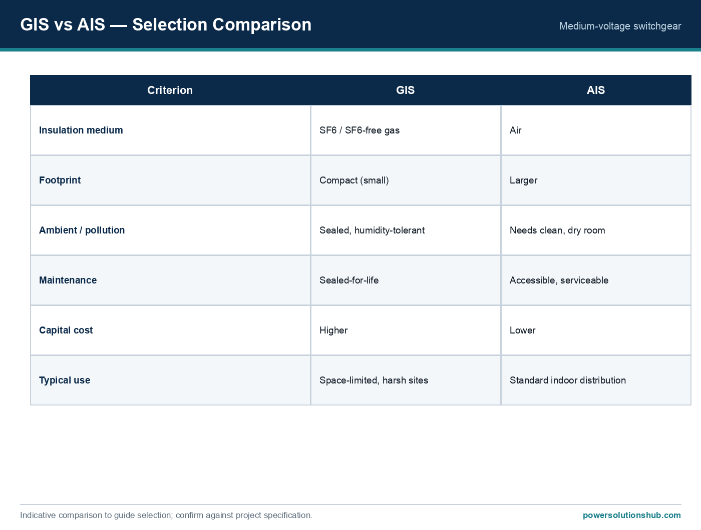
MV Cable Termination Types

MV Cable Termination Types: Heat-Shrink, Cold-Shrink and Push-On Compared

An MV cable termination is the engineered interface at the end of a medium-voltage power cable that controls electrical stress, seals out moisture, and provides a safe mechanical and electrical connection to switchgear, transformers, or overhead lines — the three dominant technologies used to build this interface are heat-shrink, cold-shrink, and push-on (slip-on) terminations. This guide explains the underlying electrical-stress-control physics, how to size and select a termination class for a given cable and voltage, walks through a worked example of calculating the maximum operating stress at the cable screen cut-back point, and compares the three technologies against installation, environmental, and maintenance criteria relevant to buyers across the Middle East and Gulf region (including Egypt and Saudi Arabia), North Africa, the CIS, and Sub-Saharan Africa.

Choosing the wrong termination type is one of the most common root causes of MV cable failures in the field — not because the cable itself is deficient, but because uncontrolled electrical stress at the screen cut-back point initiates partial discharge, tracking, and eventual flashover. Understanding the stress-control method behind each termination family lets engineers select correctly rather than by habit or price alone.

MV Cable Termination Types — schematic
MV Cable Termination Types — schematic.

Why Termination Design Matters: The Electrical Stress Problem

Inside a shielded MV cable, the semiconducting screen keeps the electric field radially symmetric around the conductor. The moment that screen is cut back to expose insulation for the termination, the field lines are no longer confined — they concentrate sharply at the screen cut-off edge. This localized stress can be many times higher than the bulk stress in the cable insulation, and if left uncontrolled it will initiate partial discharge activity, erosion, and eventual dielectric breakdown.

All three termination technologies exist to solve this one problem, using two alternative approaches:

  • Geometric (stress-cone) control — physically increasing the insulation thickness and radius at the cut-back point to spread the field over a larger volume, lowering the local gradient.
  • Capacitive (stress-control tube/mastic) control — using a high-permittivity semiconducting or capacitive-graded material sleeve that redistributes the field axially along a longer path instead of concentrating it at a point.

Heat-shrink, cold-shrink, and push-on terminations all deliver one of these two stress-control mechanisms, just through different installation methods and material systems.

Selection reference
Selection reference.

The Method: Electrical Stress Formula and Sizing Logic

The starting point for any termination engineering check is the electric field at the screen cut-back edge, approximated using the coaxial cylindrical capacitor stress formula:

E = V / [r × ln(R/r)]

Where: – E = electric field stress at the inner radius (kV/mm) – V = phase-to-ground voltage applied across the insulation (kV) – r = radius of the conductor/screen cut-back point (mm) – R = outer radius of the insulation (mm) – ln = natural logarithm

Without stress control, the field at the screen edge approaches a near-singular concentration because the effective “r” at that sharp edge becomes very small, driving E toward very high values. A stress cone or stress-control tube effectively increases the local radius of curvature and/or the effective dielectric path length, which — because E is inversely proportional to r and to ln(R/r) — directly reduces the peak gradient to a manageable level.

The selection logic for a termination therefore follows three sizing checks:

  1. Voltage class match — the termination’s rated voltage and rated lightning-impulse withstand must meet or exceed the cable system’s rated voltage class and insulation level.
  2. Conductor size range — every termination kit covers a specific cable conductor cross-section and insulation diameter window; installing outside that window compromises the stress-control geometry.
  3. Creepage distance for environment — outdoor terminations in polluted, coastal, or desert-dust environments need longer creepage paths (achieved via sheds/skirts) than indoor terminations in a clean switchgear cubicle.

Worked Example: Stress Reduction With a Stress Cone

Consider an 11 kV system (phase-to-ground voltage ≈ 6.35 kV, since V_phase = V_line/√3 = 11/1.732 ≈ 6.35 kV) terminating a cable with a conductor-plus-insulation screen cut-back radius of r = 10 mm and an outer insulation radius at the stress-control point of R = 14 mm.

Step 1 — Stress without any control (approximated at the sharp screen edge): If the effective radius at the sharp cut edge is very small — say r_edge ≈ 1 mm — the stress approximates to:

E_uncontrolled ≈ V / [r_edge × ln(R/r_edge)] = 6.35 / [1 × ln(14/1)] = 6.35 / ln(14) = 6.35 / 2.64 ≈ 2.4 kV/mm

Step 2 — Stress with a stress cone applied (effective radius increased to r = 10 mm, R = 14 mm):

E_controlled = V / [r × ln(R/r)] = 6.35 / [10 × ln(14/10)] = 6.35 / [10 × 0.336] = 6.35 / 3.36 ≈ 1.89 kV/mm

Step 3 — Compare: Even this simplified calculation shows the stress-cone geometry pulling the peak field down toward the bulk cable insulation stress level, rather than the sharp, highly localized multiplication that occurs at an unprotected screen cut edge. In practice, the uncontrolled edge stress is far more concentrated than this illustrative flat comparison suggests (real field solutions use finite-element analysis), but the first-principles direction is clear: increasing the effective radius and dielectric path length at the screen termination point is what a stress cone, a heat-shrink stress tube, or a cold-shrink body is engineered to achieve.

This is why every reputable termination kit datasheet specifies an exact cable conductor and insulation diameter range — the stress-control component is only effective within its designed geometric window.

Comparison Table: Heat-Shrink vs Cold-Shrink vs Push-On

Criterion Heat-Shrink Cold-Shrink Push-On (Slip-On)
Stress-control method Heat-applied tube with integral stress-control mastic/tube Pre-expanded elastomeric tube removed from a core, self-shrinks onto cable Pre-molded elastomeric body with factory-built stress cone, pushed directly onto prepared cable
Installation tool Propane torch / heat gun required No heat source needed — mechanical removal of support core Lubricant and mechanical push force; sometimes a installation tool for larger sizes
Skill sensitivity Moderate–high (uneven heating risks voids/wrinkles) Low–moderate (core-pull technique, but dimensionally forgiving) Low–moderate (requires accurate dimensional prep, tight tolerance fit)
Hot-work / fire permit needed Yes (open flame or hot-air gun) No No
Typical best fit Outdoor/indoor terminations where flexible kits across a wide diameter range are desired Indoor and outdoor terminations in hazardous areas, confined spaces, or where hot work is restricted Factory-engineered, consistent repeatable installs; common for separable connectors at switchgear bushings
Field rework/removability Difficult — material is cross-linked after shrinking Difficult — once relaxed onto cable, not designed for reuse Can be de-installed and reinstalled more readily in some designs
Dimensional tolerance to cable variation Wide (shrinks down, accommodates range) Wide (pre-expanded to a large diameter) Narrower — must match molded body ID closely
Common application Overhead-to-cable transitions, retrofit terminations, pole-mounted equipment Switchgear compartments, confined vaults, ATEX/hazardous zones Transformer bushings, switchgear cable boxes, separable elbow connectors

Selection Criteria and Common Pitfalls

1. Match the voltage class and BIL, not just the cable voltage rating. A termination must be rated for the system’s lightning-impulse withstand level and continuous voltage, not just the nominal cable voltage printed on the drum.

2. Verify the conductor and insulation diameter window. Every stress-control component (cone, tube, or molded body) is only effective within its designed diameter range — installing a kit outside its window is a leading cause of premature termination failure, regardless of which of the three technologies is chosen.

3. Account for indoor vs outdoor creepage requirements. Outdoor terminations exposed to pollution, salt fog, or desert dust need additional creepage distance via sheds; indoor terminations inside a clean, dry switchgear cubicle typically need less.

4. Consider site conditions and hot-work restrictions. Cold-shrink and push-on technologies avoid open-flame or hot-air installation, which matters in hazardous-area work, confined cable vaults, or sites where hot-work permits are difficult to obtain. Heat-shrink remains popular where its wide dimensional tolerance and lower kit cost outweigh the need for a controlled heating tool and trained installer.

5. Don’t ignore screen bonding and grounding. Whichever termination technology is used, the cable’s metallic screen must still be correctly bonded and grounded per the cable’s screen-bonding scheme (single-point, both-ends, or cross-bonded) — the termination kit does not substitute for correct screen earthing design.

6. Confirm compatibility with the switchgear’s cable box or bushing. Terminations ultimately connect into switchgear cable compartments, transformer bushings, or ring main unit cable chambers — refer to the governing MV switchgear and transformer technical guides to verify clearance, IP rating, and interface compatibility before specifying a termination kit.

7. Protection coordination is a separate, downstream check. A correctly stress-controlled termination reduces the risk of a fault originating at the cable end, but overall system protection — fed by MV protection relays — must still be coordinated to clear any downstream fault quickly and selectively.

Standards and Compliance

Medium-voltage cable accessories, including heat-shrink, cold-shrink, and push-on terminations, are governed internationally primarily under the IEC 60502 series for power cables with extruded insulation and their accessories, and under IEC 60840 / IEC 62067 for higher-voltage extruded cable systems where applicable to the voltage class. Cable termination and joint test methods and type-test requirements are also commonly referenced against CENELEC HD 629 and relevant national adoptions in different export markets. Projects in the Middle East, North Africa, CIS, and Sub-Saharan Africa frequently specify compliance to the IEC series above alongside local utility or EPC-specific accessory qualification tests — always confirm the governing standard and test certificate with the manufacturer’s type-test report rather than assuming blanket conformity.

Related guides

See also our guides on medium voltage switchgear, gas-insulated switchgear and metal-clad switchgear.

What is the main difference between heat-shrink and cold-shrink MV terminations?

Heat-shrink terminations require a heat source (torch or heat gun) to shrink a tube with integral stress-control material onto the cable, while cold-shrink terminations are pre-expanded onto a removable core and shrink into place mechanically once the core is pulled out, requiring no heat.

Which termination type is best for hazardous or confined areas?

Cold-shrink and push-on terminations are generally preferred in hazardous areas or confined cable vaults because they avoid the open flame or hot-air tooling required for heat-shrink installation.

Do all three termination types provide the same level of electrical stress control?

All three are engineered to control the electric field concentration at the cable screen cut-back point, either through geometric stress-cone shaping or capacitive stress-control materials — but the effectiveness depends on installing the correct kit within its designed cable diameter and voltage range, not on the technology family alone.

Can a push-on termination be reused after removal?

Some push-on/separable designs allow de-installation and reinstallation more readily than heat-shrink or cold-shrink types, which are generally not designed for reuse once installed, but this varies by product design and should be confirmed with the manufacturer.

How do I size a termination for a given cable?

Match the termination’s rated voltage class and lightning-impulse withstand to the cable system rating, confirm the cable’s conductor and insulation diameter falls within the kit’s specified range, and select indoor or outdoor creepage class based on the installation environment.

Does the termination type affect screen bonding and grounding design?

No — screen bonding and grounding (single-point, both-ends, or cross-bonded) is a separate design decision governed by cable length and system configuration; the termination technology does not replace correct screen earthing.

What standards govern MV cable terminations?

MV cable terminations are primarily assessed against the IEC 60502 series for extruded power cable accessories, with IEC 60840/62067 applicable at higher extruded-cable voltage classes, and test methods frequently cross-referenced to CENELEC HD 629 — confirm the exact governing standard against the manufacturer’s type-test documentation.

Looking for medium voltage cable terminations?

Looking for high-quality medium voltage cable terminations? We provide expert engineering support and reliable products for all your medium voltage needs.

For quotations and requests: info@electricistanbul.com

WhatsApp: +90 501 076 69 91
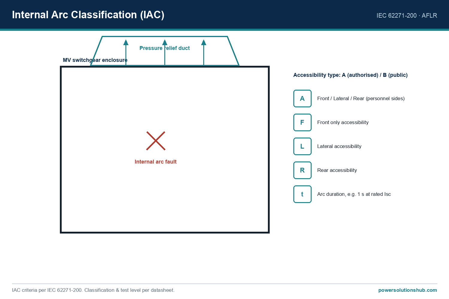
Withdrawable vs Fixed MV Switchgear

Withdrawable vs Fixed MV Switchgear: Engineering Comparison and Selection Guide

Withdrawable (draw-out) MV switchgear is a design in which the circuit breaker or contactor truck can be racked between service, test, and disconnected positions without removing the main busbar connections, while fixed (non-withdrawable) switchgear permanently bolts the switching device to the busbar and cable circuit. This guide walks through the engineering logic behind choosing one architecture over the other — isolation philosophy, maintenance access, fault-loop interruption, and a worked numerical example on service continuity and outage-time trade-offs — framed around IEC switchgear standards. It is written for specifying engineers, utility planners, and EPC buyers across the Middle East and Gulf region including Egypt and Saudi Arabia, North Africa, CIS, and Sub-Saharan Africa, where both panel types are widely deployed depending on network criticality and maintenance culture.

Readers evaluating this decision alongside related equipment should also review our hub pages on [medium voltage switchgear](/what-is-mv-switchgear-medium-voltage-switchgear/), [protection relays](/what-is-a-medium-voltage-protection-relay-mv-protection-relay/), and power transformers, since breaker type, relay coordination, and transformer protection all interact with the withdrawable/fixed choice.

Withdrawable vs Fixed MV Switchgear — schematic
Withdrawable vs Fixed MV Switchgear — schematic.

Why the Architecture Choice Matters

The core engineering question is not “which is better” in absolute terms but “what does the installation need from isolation, maintainability, and footprint.” Three first-principles factors drive the decision:

  1. Isolation integrity — can the breaker be physically separated from live busbar/cable conductors with a visible, lockable gap, without de-energizing adjacent panels?
  2. Mean time to repair (MTTR) — how fast can a faulted or tripped unit be swapped out and the feeder restored?
  3. Footprint and cost per bay — withdrawable mechanisms (racking rails, shutters, auxiliary/control plug contacts) add width, height, and component count compared to a fixed bolted connection.

These three variables are traded off against each other in every MV panel specification, and the correct answer changes with feeder criticality, spare-breaker availability, and operator skill level on site.

Selection reference
Selection reference.

The Method: How to Evaluate the Trade-off

There is no single formula that outputs “withdrawable” or “fixed” — instead, the selection method is a structured comparison across four calculable or rateable dimensions:

1. Isolation distance and dead-time. For withdrawable gear, isolation is achieved by racking the truck from “service” to “test/disconnected,” opening an air gap that meets the rated insulation level without de-energizing the busbar. For fixed gear, isolation of the same bay requires either upstream disconnection or use of a separate disconnector/earthing switch, which may require switching adjacent circuits off as well.

2. Restoration time (MTTR) after a fault or scheduled maintenance. MTTR_withdrawable ≈ t_rack-out + t_inspect/replace + t_rack-in MTTR_fixed ≈ t_de-energize-bus + t_unbolt + t_replace + t_rebolt + t_re-energize

3. Spare-unit economics. Withdrawable systems allow one spare truck to serve multiple bays of the same rating, because the truck is a modular, interchangeable unit. Fixed breakers are typically bay-specific once terminated, so spares must often be dedicated per bay type.

4. Footprint and civil cost per bay, since the racking mechanism, shutters, and auxiliary plug/socket contacts increase cubicle width and depth relative to a fixed design.

Worked Example: Outage-Time Comparison for a Feeder Bay Swap

Assume a distribution substation feeder bay needs its circuit breaker replaced after a protection trip (e.g., internal mechanical fault, not a busbar fault), and the crew must restore supply as quickly as possible.

Withdrawable case: – Time to isolate (rack breaker from service to test position): t₁ = 5 minutes – Time to withdraw faulty truck and insert spare truck: t₂ = 15 minutes – Time to rack spare truck back to service position and close: t₃ = 5 minutes – Total MTTR_withdrawable = t₁ + t₂ + t₃ = 5 + 15 + 5 = 25 minutes

Fixed case (same fault, no draw-out mechanism): – Time to de-energize and earth the busbar section serving that bay (may also affect adjacent bays sharing the section): t₁ = 20 minutes – Time to unbolt busbar/cable terminations from the faulty breaker: t₂ = 30 minutes – Time to fit, align, and rebolt the replacement breaker: t₃ = 40 minutes – Time to remove earths, re-energize, and confirm: t₄ = 15 minutes – Total MTTR_fixed = 20 + 30 + 40 + 15 = 105 minutes

Interpretation: In this illustrative scenario, the withdrawable architecture reduces restoration time by roughly (105 − 25) / 105 ≈ 76% for this specific maintenance event. This is a first-principles worked example to illustrate why withdrawable gear is specified for critical feeders — actual times vary by site access, crew training, and whether adjacent circuits must also be de-energized. The saving is largest precisely where an outage has the highest cost: hospitals, data centers, process industries, and interconnection points feeding multiple downstream transformers.

This same logic extends to rated-current sizing checks that engineers run alongside the MTTR comparison. For example, for a 1000 kVA transformer feeding the bay at a system voltage of 11 kV, the rated secondary-side current is:

I = S / (√3 × V) = 1,000,000 / (1.732 × 11,000) ≈ 52.5 A

Confirming that the replacement breaker/truck’s rated continuous current comfortably exceeds this 52.5 A feeder demand (with margin for growth) is a standard check performed regardless of whether the gear is withdrawable or fixed — the architecture choice affects how fast you can act, not what current rating you need.

Selection and Comparison Table

Criterion Withdrawable (Draw-out) Fixed (Non-withdrawable)
Isolation method Racking to test/disconnected position; visible air gap Bus/cable de-energization or separate disconnector needed
Typical MTTR for breaker swap (illustrative) ~25 min (see worked example) ~105 min (see worked example)
Spare-unit strategy One spare truck can serve multiple identical bays Spares generally bay-specific
Footprint per bay Larger (racking rails, shutters, aux contacts) Smaller, more compact
Mechanical complexity Higher (racking mechanism, interlocks, shutters) Lower (bolted, fewer moving parts)
Maintenance skill required on site Moderate (racking procedure, interlock awareness) Can be lower for routine ops, higher for breaker R&R
Best suited to Critical/continuous-process feeders, utility substations, hospitals, data centers Smaller distribution feeders, cost-sensitive projects, ring main units
Initial capital cost per bay Generally higher Generally lower

Note: the MTTR figures above are illustrative, scenario-specific numbers from the worked example, not vendor-published specifications — actual times depend on site layout, crew competency, and whether the gear includes remote racking or motorized mechanisms.

Selection Criteria and Common Pitfalls

When withdrawable gear is the right call: – Feeders where unplanned outage cost is high (hospitals, data centers, oil & gas, continuous process lines). – Substations where fast fault recovery and minimal disturbance to adjacent bays are operational requirements. – Sites with trained maintenance crews familiar with racking interlocks and safe isolation procedures.

When fixed switchgear is acceptable or preferable: – Smaller distribution substations or ring main units where simplicity, lower footprint, and lower capital cost outweigh fast-swap convenience. – Applications where the switching device (e.g., ring main unit with load-break switches) is not expected to be frequently removed for maintenance. – Projects where budget constraints dominate and planned maintenance windows are acceptable.

Common pitfalls: – Specifying withdrawable gear without budgeting for spare trucks — the fast-MTTR benefit disappears if no spare unit exists on site. – Ignoring interlock design: racking interlocks must prevent insertion/withdrawal under load or with earthing switches closed, in line with IEC safety interlocking requirements. – Assuming withdrawable gear is always “better” — for small, non-critical feeders, the added footprint and cost of draw-out mechanisms may not be justified. – Overlooking shutter and IP-rating details: withdrawable compartments rely on automatic safety shutters to cover live busbar contacts when the truck is withdrawn, and this shutter mechanism itself needs maintenance. – Failing to coordinate the breaker’s rated short-circuit breaking current, rated current, and insulation level with the actual network study — architecture (withdrawable vs fixed) does not substitute for correct electrical rating selection, which should follow IEC 62271-100 (high-voltage alternating-current circuit-breakers) and the general common specifications of IEC 62271-1 (common specifications for high-voltage switchgear and controlgear).

Standards

MV switchgear construction, type testing, and classification — including requirements relevant to withdrawable (draw-out) and fixed-mounted circuit-breaker assemblies — fall under the IEC 62271 series: IEC 62271-1 sets common specifications for high-voltage switchgear and controlgear, and IEC 62271-100 covers high-voltage alternating-current circuit-breakers including their rated characteristics and type tests. Internal arc classification (IAC) and metal-enclosed switchgear requirements are addressed within the same family of standards and should be confirmed against the specific equipment datasheet rather than assumed generically.

Related guides

See also our guides on gas-insulated switchgear, metal-clad switchgear and air-insulated switchgear.

What is the main functional difference between withdrawable and fixed MV switchgear?

Withdrawable switchgear allows the circuit breaker or contactor truck to be racked out to a test or disconnected position for maintenance without de-energizing the busbar, while fixed switchgear has the switching device permanently bolted in place, requiring upstream isolation to work on it safely.

Does withdrawable switchgear always have a shorter outage time than fixed switchgear?

In the general case, yes, for breaker replacement or maintenance events, because racking avoids unbolting live connections — as illustrated in the worked MTTR example above — but actual times depend on site conditions, crew skill, and whether a spare truck is available.

Is withdrawable switchgear more expensive than fixed switchgear?

Generally yes, per bay, because of the added racking mechanism, interlocks, shutters, and auxiliary plug/socket contacts; the extra cost is justified when fast restoration and operational flexibility have high value, such as on critical feeders.

Can fixed switchgear still meet high reliability requirements?

Yes — fixed switchgear can be highly reliable for its intended duty, particularly in smaller distribution networks or ring main units where the switching device is rarely removed; reliability depends more on correct electrical rating, protection coordination, and maintenance regime than on architecture alone.

What interlocks are required for withdrawable switchgear?

Racking interlocks must prevent the truck from being inserted into or withdrawn from the service position while the breaker is closed or carrying load, and must coordinate with earthing-switch position to prevent unsafe operation — interlock philosophy is governed by the general switchgear standards referenced above.

How do I decide between withdrawable and fixed for a new substation design?

Compare feeder criticality, available maintenance skill and spare-unit budget, footprint constraints, and capital cost against the illustrative MTTR method shown in this guide, then confirm the final electrical ratings (current, short-circuit, insulation level) independently of the architecture decision.

Does the withdrawable vs fixed choice affect protection relay coordination?

Not directly — protection relay settings are determined by fault-current studies and time-current coordination, not by breaker mounting type; however, withdrawable designs often include auxiliary contacts that signal truck position to the protection and control system, which should be accounted for in the relay’s interlocking logic. See our [protection relays](/protection-relays) hub page for related coordination guidance.

Looking for medium voltage switchgear?

Looking for high-quality medium voltage switchgear? We provide expert engineering support and reliable products for all your medium voltage needs.

For quotations and requests: info@electricistanbul.com

WhatsApp: +90 501 076 69 91